GEV Bayesian Inference with Adjustment for Missing Data

Performs Bayesian inference using a GEV distribution using block maxima, with the option to make an adjustment for the numbers of non-missing raw values in each block.

Usage

gev_bayes(
  data,
  block_length,
  block,
  adjust = TRUE,
  discard = 0,
  init = "quartiles",
  prior = revdbayes::set_prior(prior = "flat", model = "gev"),
  n = 1000,
  ...
)

Arguments

data

Either

a numeric vector containing a time series of raw data,
an object returned from block_maxima, a list with components maxima, notNA and n,
a data frame or named list containing the same information, that is, the variables maxima, notNA and n, as an object returned from block_maxima, such as the data frame BrestSurgeMaxima.

block_length

A numeric scalar. Used calculate the maxima of disjoint blocks of block_length contiguous values in the vector data. If length(data) is not an integer multiple of block_length then the values at the end of data that do not constitute a complete block of length block_length are discarded, without warning.

block

A numeric vector with the same length as data. The value of block[i] indicates the block into which data[i] falls. For example, block could provide the year in which observation i was observed.

adjust

A logical scalar or a numeric scalar in [0, 100].

If adjust = TRUE then the adjustment, described in Details, for the numbers of non-missing values underlying each block maximum is performed.
If adjust = FALSE then no adjustment is made, that is, the block maxima are treated as if the underlying raw data have no missing values.

discard

A numeric scalar. Any block maximum for which greater than discard percent of the underlying raw values were missing is discarded. Whether or not an adjustment for missingness is made for the block maxima that remain is determined by adjust.

init

Either a character scalar, one of "quartiles" or "moments", or a numeric vector of length 3 giving initial estimates of the GEV location, scale and shape parameters: \(\mu\), \(\sigma\) and \(\xi\). If init = "quartiles" then initial estimates of \(\mu\) and \(\sigma\) are based on sample quartiles of block maxima, ignoring the underlying numbers of non-missing raw data, and a value of 0 for \(\xi\). If init = "moments" then instead we use the sample mean and variance of these maxima and an initial value of 0.1 for \(\xi\).

prior

Specifies a prior distribution for the GEV parameters. This is most easily set using revdbayes::set_prior. The default is a prior \(\pi(\mu, \sigma, \xi) \propto \sigma^{-1}\) for \(\sigma > 0\). See revdbayes::set_prior for details.

n

A non-negative integer. The number of values to simulate from the posterior distribution for \((\mu, \sigma, \xi)\).

...

Further arguments to be passed to rust::ru.

Value

An object returned from rust::ru. The following components are added to this list

model: = "gev".
data,prior: the inputs data and prior.
call: the call to gev_bayes.
maxima: the vector of block maxima used to fit the model.
notNA: the number of non-missing raw values on which the maxima in maxima are based.
n: the maximal block length, that is, the largest number of values that could have been observed in each of these blocks.
adjust: a logical scalar indicating whether or not the adjustment in the Details section of gev_mle was performed. This is TRUE only if the input argument adjust was TRUE.
adjust,discard : the values of these input arguments.

The class of the returned object is c("evpost", "ru", "bayes", "evmissing"). Objects of class "evpost" have print, summary and plot S3 methods.

Details

The likelihood described in gev_mle is combined with the prior density provided by prior to produce, up to proportionality, a posterior density for \((\mu, \sigma, \xi)\).

A function to evaluate the log-posterior is passed to rust::ru to simulate a random sample from this posterior distribution using the generalised ratio-of-uniforms method, using relocation of the mode of the density to the origin to increase efficiency. The value of init is used as an initial estimate in a search for the posterior mode. Arguments to rust::ru can be passed via .... The default setting is trans = "none", that is, no transformation of the margins, and rotate = TRUE, rotation of the parameter axes to improve isotropy with a view to increasing efficiency.

Examples

## Simulate data with missing values

set.seed(24032025)
blocks <- 50
block_length <- 365

# Simulate raw data from an exponential distribution
sdata <- sim_data(blocks = blocks, block_length = block_length)

block_length <- sdata$block_length
# Sample from the posterior based on block maxima from full data
post1 <- gev_bayes(sdata$data_full, block_length = block_length)
summary(post1)
#> ru bounding box:  
#>                box        vals1       vals2        vals3 conv
#> a        1.0000000  0.000000000  0.00000000  0.000000000    0
#> b1minus -0.2247368 -0.429004846  0.15974262 -0.110371644    0
#> b2minus -0.1621321 -0.019225412 -0.24818777  0.008851358    0
#> b3minus -0.1642482 -0.029047475  0.12881751 -0.250596916    0
#> b1plus   0.1879785  0.313252280  0.05827902 -0.054719278    0
#> b2plus   0.2363722 -0.006931975  0.44374854  0.063496607    0
#> b3plus   0.2210291 -0.022860500  0.15366682  0.392587554    0
#> 
#> estimated probability of acceptance:  
#> [1] 0.3014772
#> 
#> sample summary 
#>        mu            sigma              xi          
#>  Min.   :5.293   Min.   :0.8603   Min.   :-0.26108  
#>  1st Qu.:5.752   1st Qu.:1.1560   1st Qu.: 0.02199  
#>  Median :5.891   Median :1.2526   Median : 0.10351  
#>  Mean   :5.892   Mean   :1.2722   Mean   : 0.10836  
#>  3rd Qu.:6.023   3rd Qu.:1.3770   3rd Qu.: 0.18551  
#>  Max.   :6.622   Max.   :2.1174   Max.   : 0.55320  

# Sample with adjustment for the number of non-missing values per block
post2 <- gev_bayes(sdata$data_miss, block_length = block_length)
summary(post2)
#> ru bounding box:  
#>                box        vals1       vals2       vals3 conv
#> a        1.0000000  0.000000000  0.00000000  0.00000000    0
#> b1minus -0.2097759 -0.401170205  0.13635852 -0.09914656    0
#> b2minus -0.1494487 -0.022968875 -0.22890427  0.01842038    0
#> b3minus -0.1581289 -0.032708269  0.10926826 -0.24677015    0
#> b1plus   0.1721255  0.286609292  0.06011017 -0.05124685    0
#> b2plus   0.2234551 -0.007772628  0.43820186  0.12479461    0
#> b3plus   0.2014593 -0.045204764  0.14281383  0.35926041    0
#> 
#> estimated probability of acceptance:  
#> [1] 0.2907822
#> 
#> sample summary 
#>        mu            sigma              xi          
#>  Min.   :5.280   Min.   :0.8527   Min.   :-0.18637  
#>  1st Qu.:5.691   1st Qu.:1.0868   1st Qu.: 0.09059  
#>  Median :5.824   Median :1.1877   Median : 0.16830  
#>  Mean   :5.832   Mean   :1.2026   Mean   : 0.17431  
#>  3rd Qu.:5.978   3rd Qu.:1.2979   3rd Qu.: 0.25386  
#>  Max.   :6.691   Max.   :1.8310   Max.   : 0.62626  

# Do not make the adjustment
post3 <- gev_bayes(sdata$data_miss, block_length = block_length,
                   adjust = FALSE)
summary(post3)
#> ru bounding box:  
#>                box       vals1       vals2        vals3 conv
#> a        1.0000000  0.00000000  0.00000000  0.000000000    0
#> b1minus -0.2082312 -0.40085910  0.14744745 -0.103149590    0
#> b2minus -0.1478147 -0.01954635 -0.22582419  0.005746205    0
#> b3minus -0.1562453 -0.03627886  0.11614224 -0.243488523    0
#> b1plus   0.1704187  0.28270962  0.05796295 -0.045892040    0
#> b2plus   0.2170089 -0.02254364  0.40616047  0.037048161    0
#> b3plus   0.2016273 -0.03106869  0.12799587  0.361525655    0
#> 
#> estimated probability of acceptance:  
#> [1] 0.2963841
#> 
#> sample summary 
#>        mu            sigma              xi         
#>  Min.   :4.793   Min.   :0.7996   Min.   :-0.1796  
#>  1st Qu.:5.326   1st Qu.:1.0626   1st Qu.: 0.0812  
#>  Median :5.461   Median :1.1525   Median : 0.1511  
#>  Mean   :5.460   Mean   :1.1667   Mean   : 0.1620  
#>  3rd Qu.:5.583   3rd Qu.:1.2562   3rd Qu.: 0.2332  
#>  Max.   :6.128   Max.   :1.6993   Max.   : 0.5507  

# Remove all block maxima with greater than 25% missing values and
# do not make the adjustment
post4 <- gev_bayes(sdata$data_miss, block_length = block_length,
                   adjust = FALSE, discard = 25)
summary(post4)
#> ru bounding box:  
#>                box       vals1      vals2       vals3 conv
#> a        1.0000000  0.00000000  0.0000000  0.00000000    0
#> b1minus -0.4182415 -1.10654891  0.4865155 -0.30734329    0
#> b2minus -0.1955913 -0.03971873 -0.2912431  0.02574945    0
#> b3minus -0.2198241 -0.12004301  0.2127574 -0.34472904    0
#> b1plus   0.2516484  0.44696188  0.1351107 -0.14020089    0
#> b2plus   0.3656681 -0.06477154  0.8800835  0.33944115    0
#> b3plus   0.3040806 -0.09814424  0.2208264  0.57640392    0
#> 
#> estimated probability of acceptance:  
#> [1] 0.2318572
#> 
#> sample summary 
#>        mu            sigma              xi         
#>  Min.   :4.704   Min.   :0.5289   Min.   :-0.2197  
#>  1st Qu.:5.227   1st Qu.:0.9553   1st Qu.: 0.2562  
#>  Median :5.391   Median :1.1013   Median : 0.4027  
#>  Mean   :5.406   Mean   :1.1407   Mean   : 0.4197  
#>  3rd Qu.:5.561   3rd Qu.:1.2873   3rd Qu.: 0.5627  
#>  Max.   :6.471   Max.   :2.3790   Max.   : 1.5490  

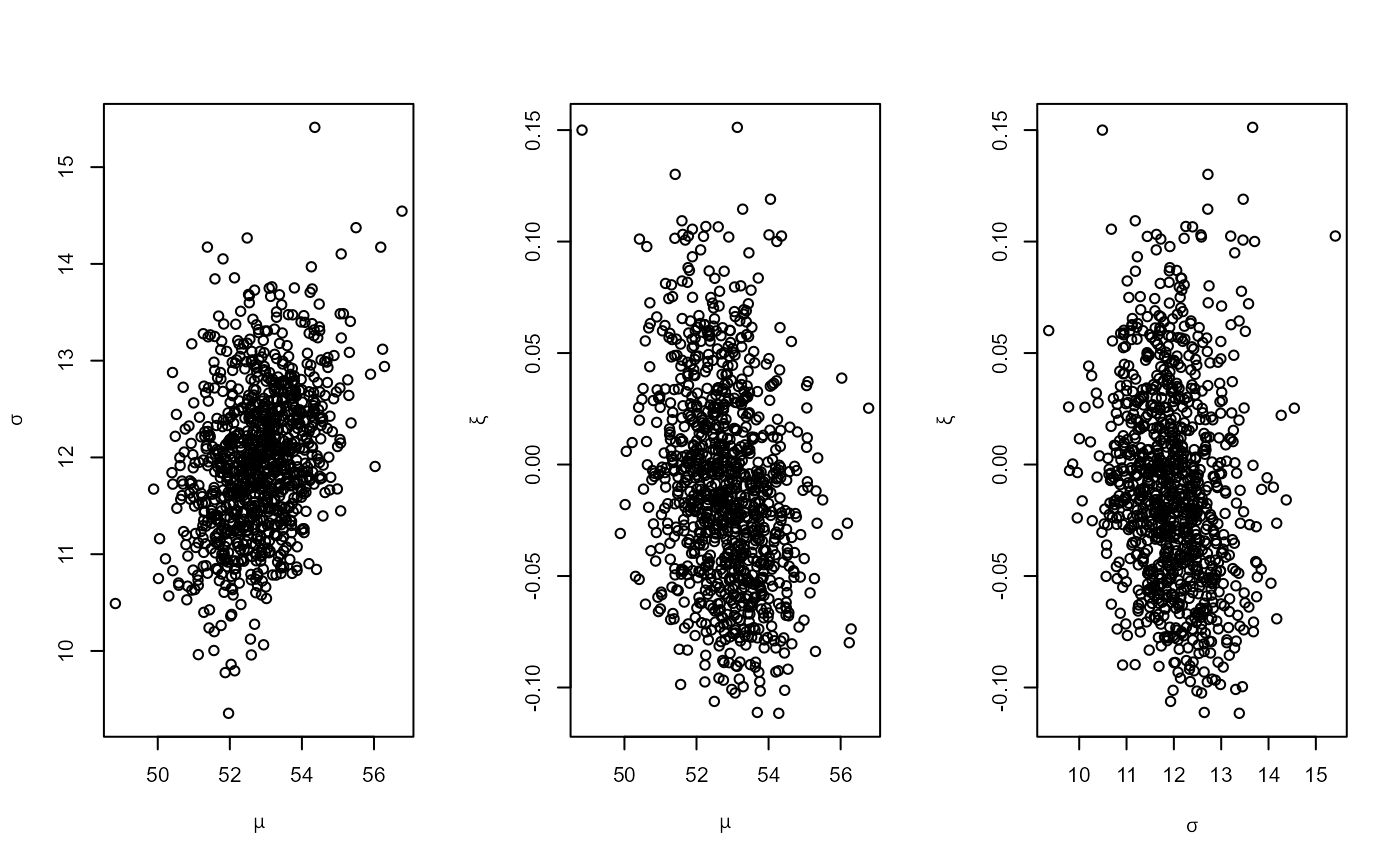
## Brest sea surge data

post <- gev_bayes(BrestSurgeMaxima)
summary(post)
#> ru bounding box:  
#>                box        vals1       vals2       vals3 conv
#> a        1.0000000  0.000000000  0.00000000  0.00000000    0
#> b1minus -0.4425320 -0.751499782  0.11680655 -0.06029664    0
#> b2minus -0.3842978 -0.021900294 -0.60490474  0.01227180    0
#> b3minus -0.3366002 -0.005334382  0.16770844 -0.49572108    0
#> b1plus   0.4169404  0.684808686  0.08450646 -0.03839377    0
#> b2plus   0.4752004 -0.024717120  0.83310983  0.02835543    0
#> b3plus   0.5203804 -0.003671959  0.20143312  0.93945441    0
#> 
#> estimated probability of acceptance:  
#> [1] 0.3097893
#> 
#> sample summary 
#>        mu            sigma              xi          
#>  Min.   :48.82   Min.   : 9.356   Min.   :-0.11157  
#>  1st Qu.:52.08   1st Qu.:11.463   1st Qu.:-0.04350  
#>  Median :52.78   Median :11.947   Median :-0.01364  
#>  Mean   :52.80   Mean   :11.973   Mean   :-0.01034  
#>  3rd Qu.:53.48   3rd Qu.:12.455   3rd Qu.: 0.01702  
#>  Max.   :56.78   Max.   :15.411   Max.   : 0.15123  
plot(post)