Threshold \(u\) and runs parameter \(D\) diagnostic for the \(D\)-gaps estimator

Creates data for a plot to aid the choice of the threshold and run parameter \(D\) for the \(D\)-gaps estimator (see dgaps). plot.choose_ud creates the plot.

Usage

choose_ud(data, u, D = 1, inc_cens = TRUE)

Arguments

data

A numeric vector or numeric matrix of raw data. If data is a matrix then the log-likelihood is constructed as the sum of (independent) contributions from different columns. A common situation is where each column relates to a different year.

If data contains missing values then split_by_NAs is used to divide the data into sequences of non-missing values.

u, D

Numeric vectors. u is a vector of extreme value thresholds applied to data. D is a vector of values of the run parameter \(D\), as defined in Holesovsky and Fusek (2020). See dgaps for more details.

Any values in u that are greater than all the observations in data will be removed without a warning being given.

inc_cens

A logical scalar indicating whether or not to include contributions from right-censored inter-exceedance times, relating to the first and last observations. It is known that these times are greater than or equal to the time observed. If data has multiple columns then there will be right-censored first and last inter-exceedance times for each column. See Details in dgaps.

Value

An object (a list) of class c("choose_ud", "exdex") containing

imt

an object of class c("dgaps_imt", "exdex") returned from dgaps_imt.

theta

a length(u) by length(D) matrix. Element (i,j) of theta contains an object (a list) of class c("dgaps", "exdex"), a result of a call dgaps(data, u[j], D[i]) to dgaps.

Details

For each combination of threshold in u and \(D\) in D the functions dgaps and dgaps_imt are called in order to estimate \(\theta\) and to perform the information matrix test of Holesovsky and Fusek (2020).

References

Holesovsky, J. and Fusek, M. Estimation of the extremal index using censored distributions. Extremes 23, 197-213 (2020). doi:10.1007/s10687-020-00374-3

See also

dgaps for maximum likelihood estimation of the extremal index \(\theta\) using the \(D\)-gaps model.

dgaps_imt for the information matrix test under the \(D\)-gaps model

plot.choose_ud to produce the diagnostic plot.

Examples

### S&P 500 index

# Multiple thresholds and left-censoring parameters
u <- quantile(sp500, probs = seq(0.2, 0.9, by = 0.1))
imt_theta <- choose_ud(sp500, u = u, D = 1:5)
plot(imt_theta)

plot(imt_theta, uprob = TRUE)

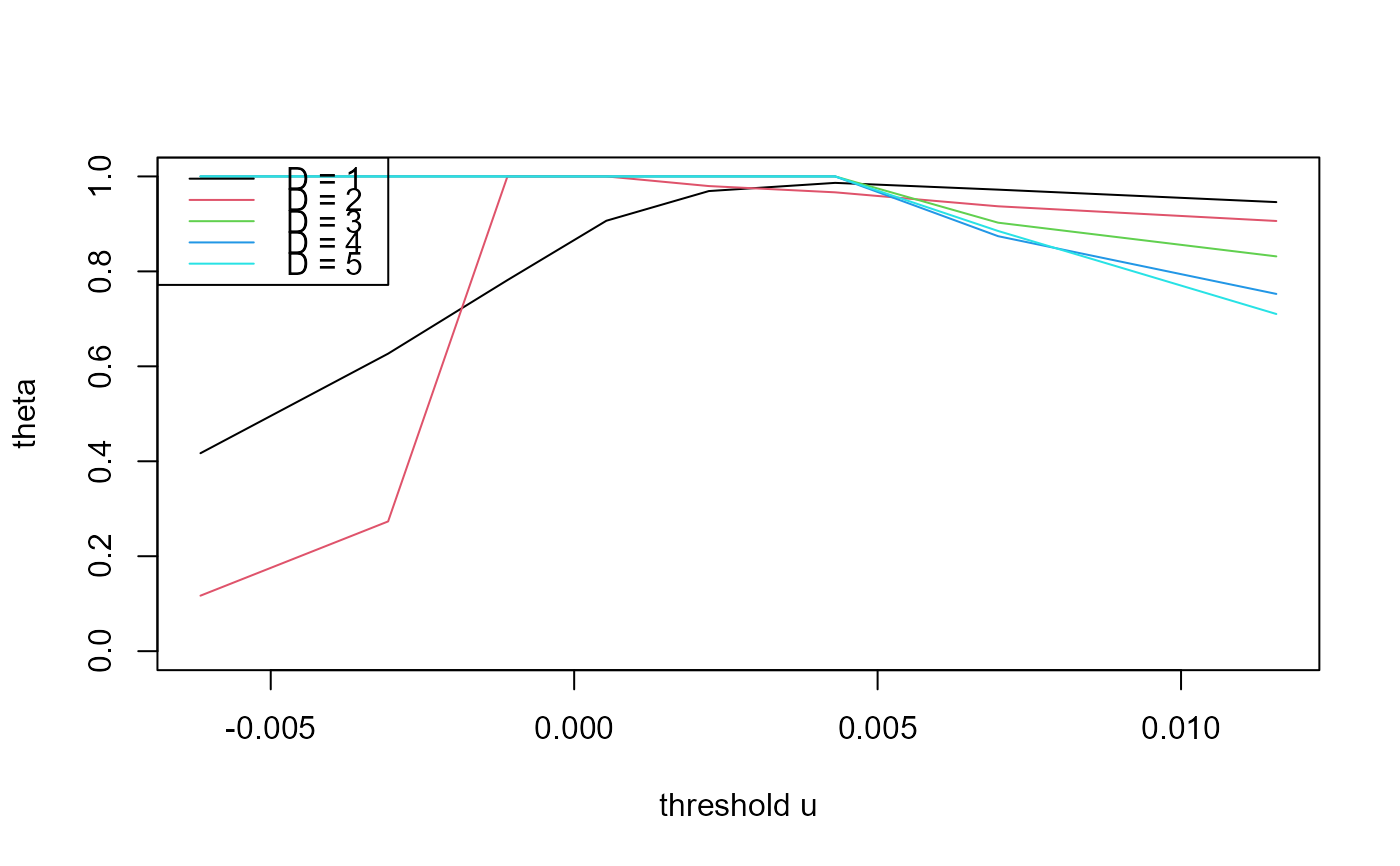
plot(imt_theta, y = "theta")


# One left-censoring parameter D, many thresholds u
u <- quantile(sp500, probs = seq(0.2, 0.9, by = 0.1))
imt_theta <- choose_ud(sp500, u = u, D = 1)
plot(imt_theta)

plot(imt_theta, y = "theta")


# One threshold u, many left-censoring parameters D
u <- quantile(sp500, probs = 0.9)
imt_theta <- choose_ud(sp500, u = u, D = 1:5)
plot(imt_theta)

plot(imt_theta, y = "theta")


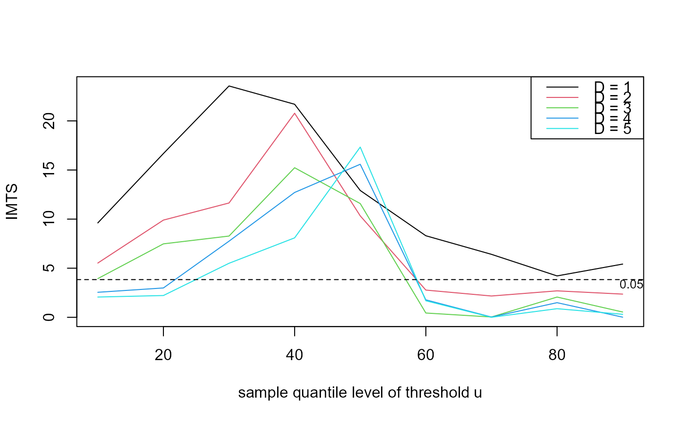
### Newlyn sea surges

u <- quantile(newlyn, probs = seq(0.1, 0.9, by = 0.1))
imt_theta <- choose_ud(newlyn, u = u, D = 1:5)
plot(imt_theta, uprob = TRUE)


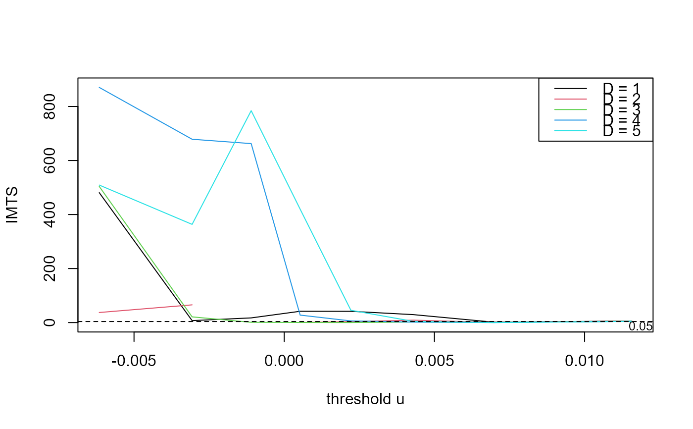
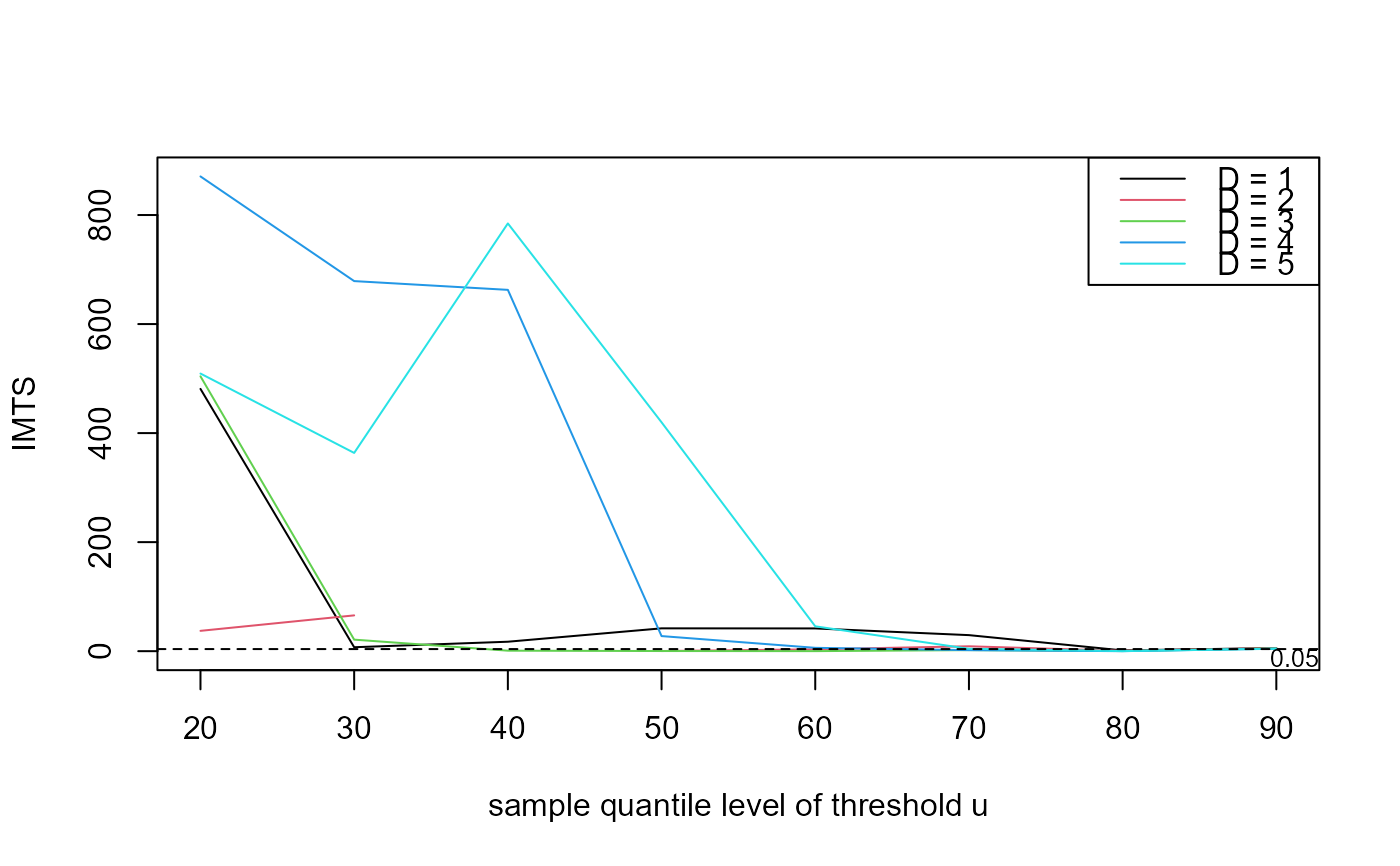
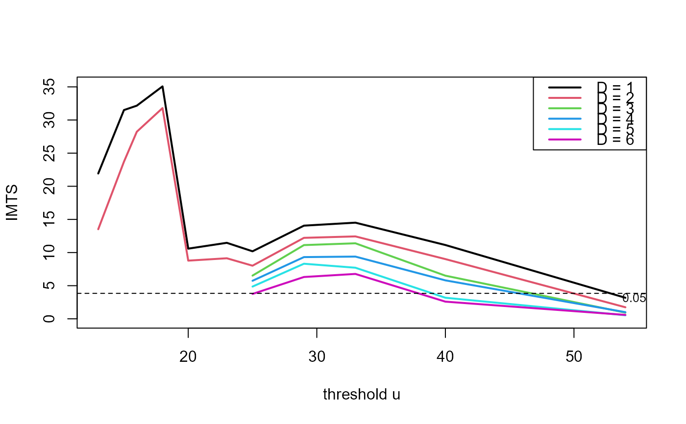
### Cheeseboro wind gusts (a matrix containing some NAs)

probs <- c(seq(0.5, 0.95, by = 0.05), 0.99)
u <- quantile(cheeseboro, probs = probs, na.rm = TRUE)
imt_theta <- choose_ud(cheeseboro, u, D = 1:6)
plot(imt_theta, uprob = FALSE, lwd = 2)


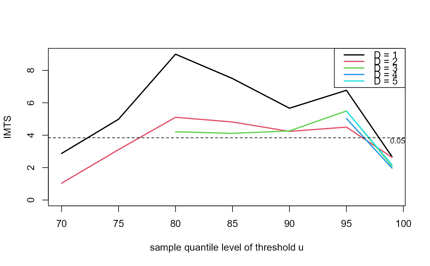
### Uccle July temperatures

probs <- c(seq(0.7, 0.95, by = 0.05), 0.99)
u <- quantile(uccle720m, probs = probs, na.rm = TRUE)
imt_theta <- choose_ud(uccle720m, u, D = 1:5)
plot(imt_theta, uprob = TRUE, lwd = 2)