Finds a value of the Box-Cox transformation parameter lambda for which
the (positive) random variable with log-density \(\log f\) has a
density closer to that of a Gaussian random variable.
In the following we use theta (\(\theta\)) to denote the argument
of \(\log f\) on the original scale and phi (\(\phi\)) on
the Box-Cox transformed scale.
Arguments
- logf
A function returning the log of the target density \(f\).
- ...
further arguments to be passed to
logfand related functions.- d
A numeric scalar. Dimension of \(f\).
- n_grid
A numeric scalar. Number of ordinates for each variable in
phi. If this is not supplied a default value ofceiling(2501 ^ (1 / d))is used.- ep_bc
A (positive) numeric scalar. Smallest possible value of
phito consider. Used to avoid negative values ofphi.- min_phi, max_phi
Numeric vectors. Smallest and largest values of
phiat which to evaluatelogf, i.e. the range of values of phi over which to evaluatelogf. Any components inmin_phithat are not positive are set toep_bc.- which_lam
A numeric vector. Contains the indices of the components of
phithat ARE to be Box-Cox transformed.- lambda_range
A numeric vector of length 2. Range of lambda over which to optimise.
- init_lambda
A numeric vector of length 1 or
d. Initial value of lambda used in the search for the best lambda. Ifinit_lambdais a scalar thenrep(init_lambda, d)is used.- phi_to_theta
A function returning (inverse) of the transformation from
thetatophiused to ensure positivity ofphiprior to Box-Cox transformation. The argument isphiand the returned value istheta.- log_j
A function returning the log of the Jacobian of the transformation from
thetatophi, i.e. based on derivatives ofphiwith respect totheta. Takesthetaas its argument.
Value
A list containing the following components
- lambda
A numeric vector. The value of lambda.
- gm
A numeric vector. Box-Cox scaling parameter, estimated by the geometric mean of the values of
phiused in the optimisation to find the value of lambda, weighted by the values of \(f\) evaluated atphi.- init_psi
A numeric vector. An initial estimate of the mode of the Box-Cox transformed density
- sd_psi
A numeric vector. Estimates of the marginal standard deviations of the Box-Cox transformed variables.
- phi_to_theta
as detailed above (only if
phi_to_thetais supplied)- log_j
as detailed above (only if
log_jis supplied)
Details
The general idea is to evaluate the density \(f\) on a
d-dimensional grid, with n_grid ordinates for each of the
d variables.
We treat each combination of the variables in the grid as a data point
and perform an estimation of the Box-Cox transformation parameter
lambda, in which each data point is weighted by the density
at that point. The vectors min_phi and max_phi define the
limits of the grid and which_lam can be used to specify that only
certain components of phi are to be transformed.
References
Box, G. and Cox, D. R. (1964) An Analysis of Transformations. Journal of the Royal Statistical Society. Series B (Methodological), 26(2), 211-252.
Andrews, D. F. and Gnanadesikan, R. and Warner, J. L. (1971) Transformations of Multivariate Data, Biometrics, 27(4).
See also
ru and ru_rcpp to perform
ratio-of-uniforms sampling.
find_lambda_one_d and
find_lambda_one_d_rcpp to produce (somewhat) automatically
a list for the argument lambda of ru/ru_rcpp for the
d = 1 case.
find_lambda_rcpp for a version of
find_lambda that uses the Rcpp package to improve
efficiency.
Examples
# Log-normal density ===================
# Note: the default value max_phi = 10 is OK here but this will not always
# be the case
lambda <- find_lambda(logf = dlnorm, log = TRUE)
lambda
#> $lambda
#> [1] 0.05408856
#>
#> $gm
#> [1] 0.971952
#>
#> $init_psi
#> [1] -0.05181524
#>
#> $sd_psi
#> Var1
#> 0.8614544
#>
x <- ru(logf = dlnorm, log = TRUE, d = 1, n = 1000, trans = "BC",
lambda = lambda)
# Gamma density ===================
alpha <- 1
# Choose a sensible value of max_phi
max_phi <- qgamma(0.999, shape = alpha)
# [Of course, typically the quantile function won't be available. However,
# In practice the value of lambda chosen is quite insensitive to the choice
# of max_phi, provided that max_phi is not far too large or far too small.]
lambda <- find_lambda(logf = dgamma, shape = alpha, log = TRUE,
max_phi = max_phi)
lambda
#> $lambda
#> [1] 0.2801406
#>
#> $gm
#> [1] 0.5525366
#>
#> $init_psi
#> [1] -0.2060046
#>
#> $sd_psi
#> Var1
#> 0.573372
#>
x <- ru(logf = dgamma, shape = alpha, log = TRUE, d = 1, n = 1000,
trans = "BC", lambda = lambda)
# \donttest{
# Generalized Pareto posterior distribution ===================
# Sample data from a GP(sigma, xi) distribution
gpd_data <- rgpd(m = 100, xi = -0.5, sigma = 1)
# Calculate summary statistics for use in the log-likelihood
ss <- gpd_sum_stats(gpd_data)
# Calculate an initial estimate
init <- c(mean(gpd_data), 0)
n <- 1000
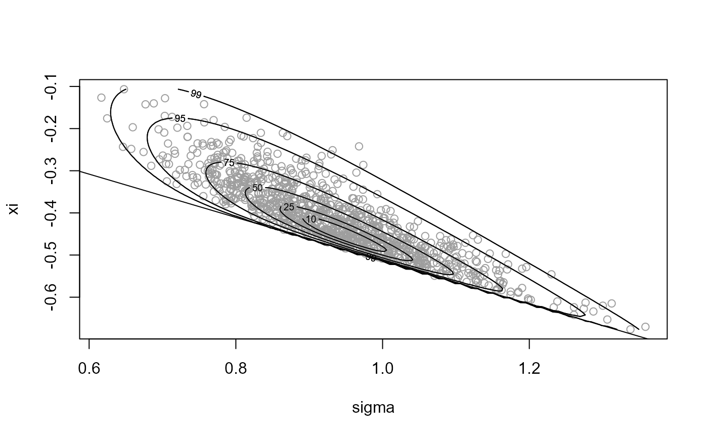
# Sample on original scale, with no rotation ----------------
x1 <- ru(logf = gpd_logpost, ss = ss, d = 2, n = n, init = init,
lower = c(0, -Inf), rotate = FALSE)
plot(x1, xlab = "sigma", ylab = "xi")
# Parameter constraint line xi > -sigma/max(data)
# [This may not appear if the sample is far from the constraint.]
abline(a = 0, b = -1 / ss$xm)
 summary(x1)
#> ru bounding box:
#> box vals1 vals2 conv
#> a 1.0000000 0.0000000 0.0000000 0
#> b1minus -0.1372312 -0.2170175 0.1428450 0
#> b2minus -0.1014964 0.3024958 -0.1777366 0
#> b1plus 0.1732783 0.3085698 -0.1800970 0
#> b2plus 0.1007068 -0.2160567 0.1800929 0
#>
#> estimated probability of acceptance:
#> [1] 0.1218324
#>
#> sample summary
#> V1 V2
#> Min. :0.7339 Min. :-0.8204
#> 1st Qu.:1.0237 1st Qu.:-0.6403
#> Median :1.1084 Median :-0.5801
#> Mean :1.1119 Mean :-0.5815
#> 3rd Qu.:1.1947 3rd Qu.:-0.5240
#> Max. :1.4858 Max. :-0.2740
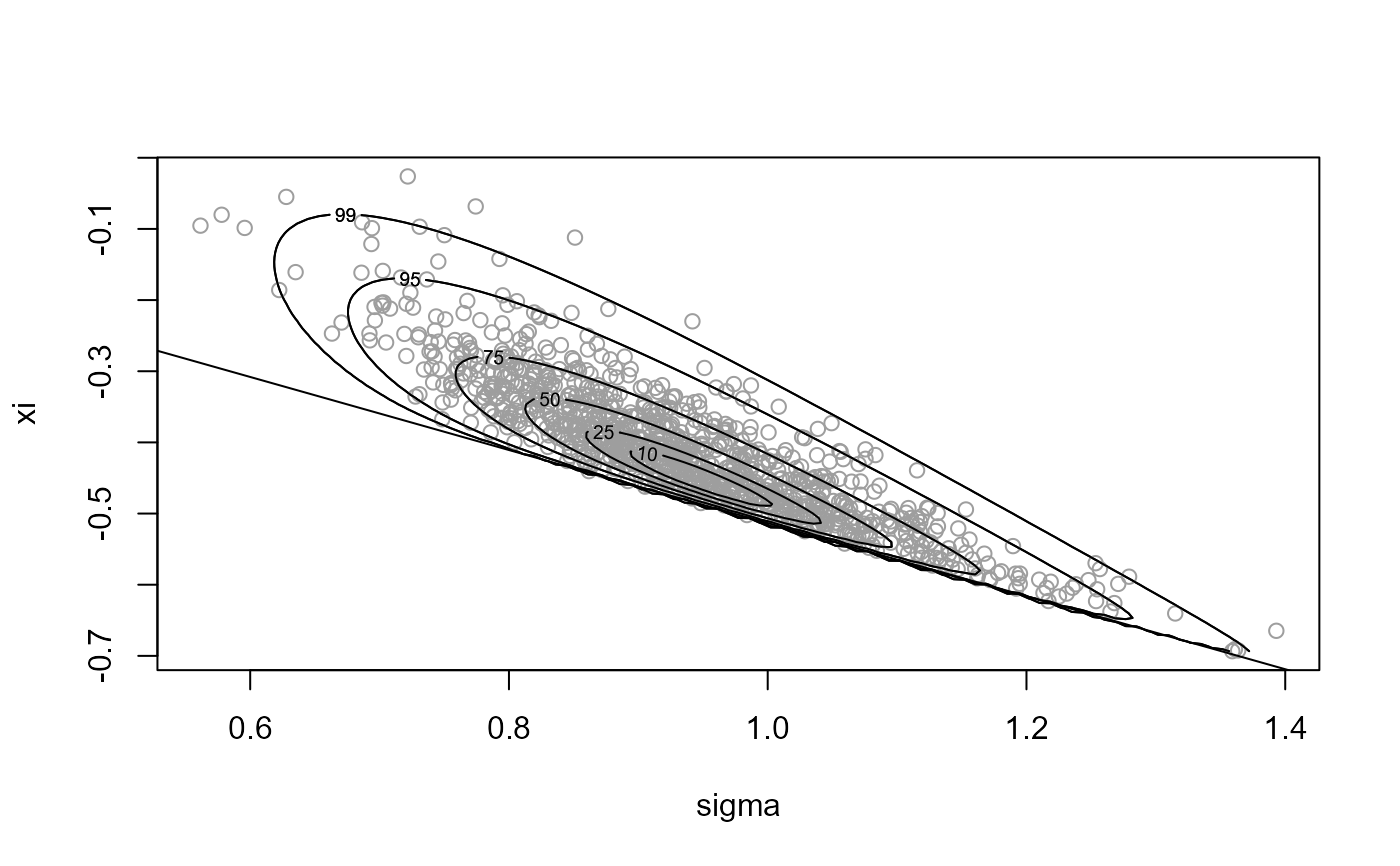
# Sample on original scale, with rotation ----------------
x2 <- ru(logf = gpd_logpost, ss = ss, d = 2, n = n, init = init,
lower = c(0, -Inf))
plot(x2, xlab = "sigma", ylab = "xi")
abline(a = 0, b = -1 / ss$xm)
summary(x1)
#> ru bounding box:
#> box vals1 vals2 conv
#> a 1.0000000 0.0000000 0.0000000 0
#> b1minus -0.1372312 -0.2170175 0.1428450 0
#> b2minus -0.1014964 0.3024958 -0.1777366 0
#> b1plus 0.1732783 0.3085698 -0.1800970 0
#> b2plus 0.1007068 -0.2160567 0.1800929 0
#>
#> estimated probability of acceptance:
#> [1] 0.1218324
#>
#> sample summary
#> V1 V2
#> Min. :0.7339 Min. :-0.8204
#> 1st Qu.:1.0237 1st Qu.:-0.6403
#> Median :1.1084 Median :-0.5801
#> Mean :1.1119 Mean :-0.5815
#> 3rd Qu.:1.1947 3rd Qu.:-0.5240
#> Max. :1.4858 Max. :-0.2740
# Sample on original scale, with rotation ----------------
x2 <- ru(logf = gpd_logpost, ss = ss, d = 2, n = n, init = init,
lower = c(0, -Inf))
plot(x2, xlab = "sigma", ylab = "xi")
abline(a = 0, b = -1 / ss$xm)
 summary(x2)
#> ru bounding box:
#> box vals1 vals2 conv
#> a 1.00000000 0.00000000 0.00000000 0
#> b1minus -0.03563256 -0.05170400 0.03652177 0
#> b2minus -0.05930462 0.03605754 -0.10385194 0
#> b1plus 0.11679615 0.27278171 0.09170647 0
#> b2plus 0.05884325 0.11826313 0.10522871 0
#>
#> estimated probability of acceptance:
#> [1] 0.4201681
#>
#> sample summary
#> V1 V2
#> Min. :0.7836 Min. :-0.8475
#> 1st Qu.:1.0361 1st Qu.:-0.6430
#> Median :1.1119 Median :-0.5870
#> Mean :1.1225 Mean :-0.5872
#> 3rd Qu.:1.2033 3rd Qu.:-0.5364
#> Max. :1.5662 Max. :-0.3164
# Sample on Box-Cox transformed scale ----------------
# Find initial estimates for phi = (phi1, phi2),
# where phi1 = sigma
# and phi2 = xi + sigma / max(x),
# and ranges of phi1 and phi2 over over which to evaluate
# the posterior to find a suitable value of lambda.
temp <- do.call(gpd_init, ss)
min_phi <- pmax(0, temp$init_phi - 2 * temp$se_phi)
max_phi <- pmax(0, temp$init_phi + 2 * temp$se_phi)
# Set phi_to_theta() that ensures positivity of phi
# We use phi1 = sigma and phi2 = xi + sigma / max(data)
phi_to_theta <- function(phi) c(phi[1], phi[2] - phi[1] / ss$xm)
log_j <- function(x) 0
lambda <- find_lambda(logf = gpd_logpost, ss = ss, d = 2, min_phi = min_phi,
max_phi = max_phi, phi_to_theta = phi_to_theta, log_j = log_j)
lambda
#> $lambda
#> [1] 0.08716679 0.34750803
#>
#> $gm
#> [1] 1.10817399 0.02472241
#>
#> $init_psi
#> [1] 0.1076681 -0.1826052
#>
#> $sd_psi
#> Var1 Var2
#> 0.12493468 0.02088563
#>
#> $phi_to_theta
#> function (phi)
#> c(phi[1], phi[2] - phi[1]/ss$xm)
#> <environment: 0x0000021bf657a140>
#>
#> $log_j
#> function (x)
#> 0
#> <environment: 0x0000021bf657a140>
#>
# Sample on Box-Cox transformed, without rotation
x3 <- ru(logf = gpd_logpost, ss = ss, d = 2, n = n, trans = "BC",
lambda = lambda, rotate = FALSE)
plot(x3, xlab = "sigma", ylab = "xi")
abline(a = 0, b = -1 / ss$xm)
summary(x2)
#> ru bounding box:
#> box vals1 vals2 conv
#> a 1.00000000 0.00000000 0.00000000 0
#> b1minus -0.03563256 -0.05170400 0.03652177 0
#> b2minus -0.05930462 0.03605754 -0.10385194 0
#> b1plus 0.11679615 0.27278171 0.09170647 0
#> b2plus 0.05884325 0.11826313 0.10522871 0
#>
#> estimated probability of acceptance:
#> [1] 0.4201681
#>
#> sample summary
#> V1 V2
#> Min. :0.7836 Min. :-0.8475
#> 1st Qu.:1.0361 1st Qu.:-0.6430
#> Median :1.1119 Median :-0.5870
#> Mean :1.1225 Mean :-0.5872
#> 3rd Qu.:1.2033 3rd Qu.:-0.5364
#> Max. :1.5662 Max. :-0.3164
# Sample on Box-Cox transformed scale ----------------
# Find initial estimates for phi = (phi1, phi2),
# where phi1 = sigma
# and phi2 = xi + sigma / max(x),
# and ranges of phi1 and phi2 over over which to evaluate
# the posterior to find a suitable value of lambda.
temp <- do.call(gpd_init, ss)
min_phi <- pmax(0, temp$init_phi - 2 * temp$se_phi)
max_phi <- pmax(0, temp$init_phi + 2 * temp$se_phi)
# Set phi_to_theta() that ensures positivity of phi
# We use phi1 = sigma and phi2 = xi + sigma / max(data)
phi_to_theta <- function(phi) c(phi[1], phi[2] - phi[1] / ss$xm)
log_j <- function(x) 0
lambda <- find_lambda(logf = gpd_logpost, ss = ss, d = 2, min_phi = min_phi,
max_phi = max_phi, phi_to_theta = phi_to_theta, log_j = log_j)
lambda
#> $lambda
#> [1] 0.08716679 0.34750803
#>
#> $gm
#> [1] 1.10817399 0.02472241
#>
#> $init_psi
#> [1] 0.1076681 -0.1826052
#>
#> $sd_psi
#> Var1 Var2
#> 0.12493468 0.02088563
#>
#> $phi_to_theta
#> function (phi)
#> c(phi[1], phi[2] - phi[1]/ss$xm)
#> <environment: 0x0000021bf657a140>
#>
#> $log_j
#> function (x)
#> 0
#> <environment: 0x0000021bf657a140>
#>
# Sample on Box-Cox transformed, without rotation
x3 <- ru(logf = gpd_logpost, ss = ss, d = 2, n = n, trans = "BC",
lambda = lambda, rotate = FALSE)
plot(x3, xlab = "sigma", ylab = "xi")
abline(a = 0, b = -1 / ss$xm)
 summary(x3)
#> ru bounding box:
#> box vals1 vals2 conv
#> a 1.00000000 0.00000000 0.00000000 0
#> b1minus -0.15141344 -0.25140461 0.02144685 0
#> b2minus -0.02701316 0.07025963 -0.04192489 0
#> b1plus 0.15401321 0.25717949 -0.01261319 0
#> b2plus 0.02844329 -0.09800733 0.04662828 0
#>
#> estimated probability of acceptance:
#> [1] 0.5162623
#>
#> sample summary
#> V1 V2
#> Min. :0.7517 Min. :-0.9308
#> 1st Qu.:1.0230 1st Qu.:-0.6388
#> Median :1.1024 Median :-0.5816
#> Mean :1.1137 Mean :-0.5837
#> 3rd Qu.:1.1957 3rd Qu.:-0.5284
#> Max. :1.7038 Max. :-0.2593
# Sample on Box-Cox transformed, with rotation
x4 <- ru(logf = gpd_logpost, ss = ss, d = 2, n = n, trans = "BC",
lambda = lambda)
plot(x4, xlab = "sigma", ylab = "xi")
abline(a = 0, b = -1 / ss$xm)
summary(x3)
#> ru bounding box:
#> box vals1 vals2 conv
#> a 1.00000000 0.00000000 0.00000000 0
#> b1minus -0.15141344 -0.25140461 0.02144685 0
#> b2minus -0.02701316 0.07025963 -0.04192489 0
#> b1plus 0.15401321 0.25717949 -0.01261319 0
#> b2plus 0.02844329 -0.09800733 0.04662828 0
#>
#> estimated probability of acceptance:
#> [1] 0.5162623
#>
#> sample summary
#> V1 V2
#> Min. :0.7517 Min. :-0.9308
#> 1st Qu.:1.0230 1st Qu.:-0.6388
#> Median :1.1024 Median :-0.5816
#> Mean :1.1137 Mean :-0.5837
#> 3rd Qu.:1.1957 3rd Qu.:-0.5284
#> Max. :1.7038 Max. :-0.2593
# Sample on Box-Cox transformed, with rotation
x4 <- ru(logf = gpd_logpost, ss = ss, d = 2, n = n, trans = "BC",
lambda = lambda)
plot(x4, xlab = "sigma", ylab = "xi")
abline(a = 0, b = -1 / ss$xm)
 summary(x4)
#> ru bounding box:
#> box vals1 vals2 conv
#> a 1.00000000 0.000000000 0.000000000 0
#> b1minus -0.06150106 -0.099778176 0.007421510 0
#> b2minus -0.06019008 -0.002424417 -0.093415996 0
#> b1plus 0.06654206 0.112194927 0.004855441 0
#> b2plus 0.06337664 -0.006219202 0.103895945 0
#>
#> estimated probability of acceptance:
#> [1] 0.5488474
#>
#> sample summary
#> V1 V2
#> Min. :0.7831 Min. :-0.8711
#> 1st Qu.:1.0316 1st Qu.:-0.6400
#> Median :1.1103 Median :-0.5837
#> Mean :1.1169 Mean :-0.5837
#> 3rd Qu.:1.1936 3rd Qu.:-0.5268
#> Max. :1.6099 Max. :-0.3284
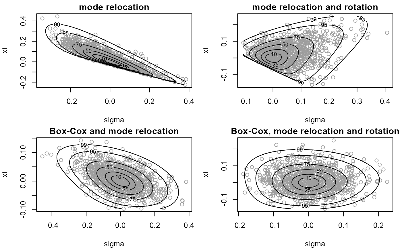
def_par <- graphics::par(no.readonly = TRUE)
par(mfrow = c(2,2), mar = c(4, 4, 1.5, 1))
plot(x1, xlab = "sigma", ylab = "xi", ru_scale = TRUE,
main = "mode relocation")
plot(x2, xlab = "sigma", ylab = "xi", ru_scale = TRUE,
main = "mode relocation and rotation")
plot(x3, xlab = "sigma", ylab = "xi", ru_scale = TRUE,
main = "Box-Cox and mode relocation")
plot(x4, xlab = "sigma", ylab = "xi", ru_scale = TRUE,
main = "Box-Cox, mode relocation and rotation")
summary(x4)
#> ru bounding box:
#> box vals1 vals2 conv
#> a 1.00000000 0.000000000 0.000000000 0
#> b1minus -0.06150106 -0.099778176 0.007421510 0
#> b2minus -0.06019008 -0.002424417 -0.093415996 0
#> b1plus 0.06654206 0.112194927 0.004855441 0
#> b2plus 0.06337664 -0.006219202 0.103895945 0
#>
#> estimated probability of acceptance:
#> [1] 0.5488474
#>
#> sample summary
#> V1 V2
#> Min. :0.7831 Min. :-0.8711
#> 1st Qu.:1.0316 1st Qu.:-0.6400
#> Median :1.1103 Median :-0.5837
#> Mean :1.1169 Mean :-0.5837
#> 3rd Qu.:1.1936 3rd Qu.:-0.5268
#> Max. :1.6099 Max. :-0.3284
def_par <- graphics::par(no.readonly = TRUE)
par(mfrow = c(2,2), mar = c(4, 4, 1.5, 1))
plot(x1, xlab = "sigma", ylab = "xi", ru_scale = TRUE,
main = "mode relocation")
plot(x2, xlab = "sigma", ylab = "xi", ru_scale = TRUE,
main = "mode relocation and rotation")
plot(x3, xlab = "sigma", ylab = "xi", ru_scale = TRUE,
main = "Box-Cox and mode relocation")
plot(x4, xlab = "sigma", ylab = "xi", ru_scale = TRUE,
main = "Box-Cox, mode relocation and rotation")
 graphics::par(def_par)
# }
graphics::par(def_par)
# }