Plot diagnostics for an ru object

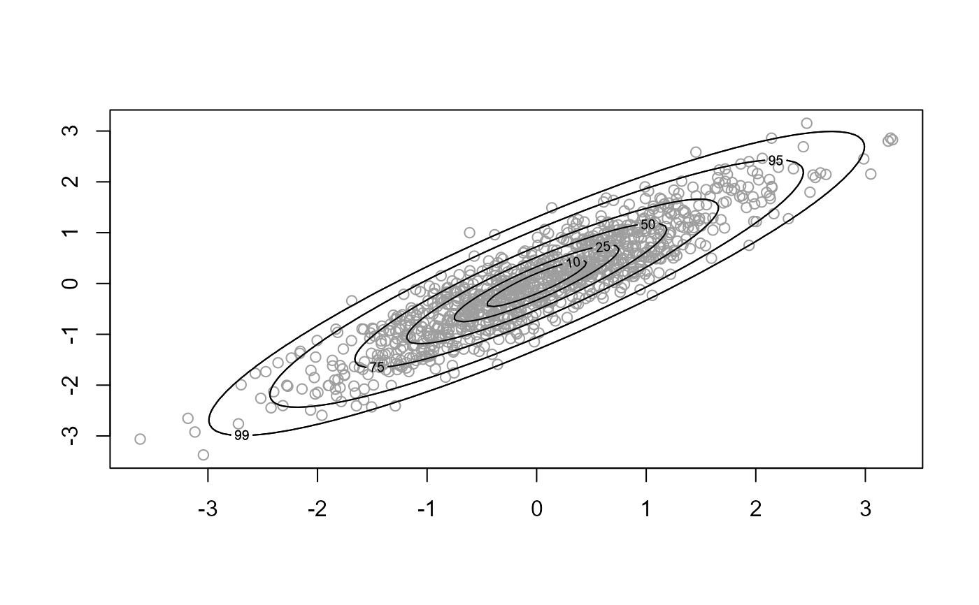
plot method for class "ru". For d = 1 a histogram of the simulated values is plotted with a the density function superimposed. The density is normalized crudely using the trapezium rule. For d = 2 a scatter plot of the simulated values is produced with density contours superimposed. For d > 2 pairwise plots of the simulated values are produced.

Usage

# S3 method for class 'ru'
plot(
  x,
  y,
  ...,
  n = ifelse(x$d == 1, 1001, 101),
  prob = c(0.1, 0.25, 0.5, 0.75, 0.95, 0.99),
  ru_scale = FALSE,
  rows = NULL,
  xlabs = NULL,
  ylabs = NULL,
  var_names = NULL,
  points_par = list(col = 8)
)

Arguments

x

an object of class "ru", a result of a call to ru.

y

Not used.

...

Additional arguments passed on to hist, lines, contour or points.

n

A numeric scalar. Only relevant if x$d = 1 or x$d = 2. The meaning depends on the value of x$d.

For d = 1 : n + 1 is the number of abscissae in the trapezium method used to normalize the density.
For d = 2 : an n by n regular grid is used to contour the density.

prob

Numeric vector. Only relevant for d = 2. The contour lines are drawn such that the respective probabilities that the variable lies within the contour are approximately equal to the values in prob.

ru_scale

A logical scalar. Should we plot data and density on the scale used in the ratio-of-uniforms algorithm (TRUE) or on the original scale (FALSE)?

rows

A numeric scalar. When d > 2 this sets the number of rows of plots. If the user doesn't provide this then it is set internally.

xlabs, ylabs

Numeric vectors. When d > 2 these set the labels on the x and y axes respectively. If the user doesn't provide these then the column names of the simulated data matrix to be plotted are used.

var_names

A character (or numeric) vector of length x$d. This argument can be used to replace variable names set using var_names in the call to ru or ru_rcpp.

points_par

A list of arguments to pass to points to control the appearance of points depicting the simulated values. Only relevant when d = 2.

Value

No return value, only the plot is produced.

Examples

# Log-normal density ----------------
x <- ru(logf = dlnorm, log = TRUE, d = 1, n = 1000, lower = 0, init = 1)
# \donttest{
plot(x)

# }
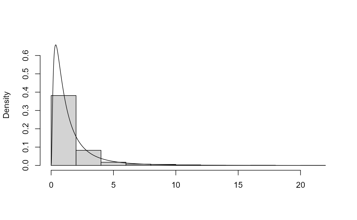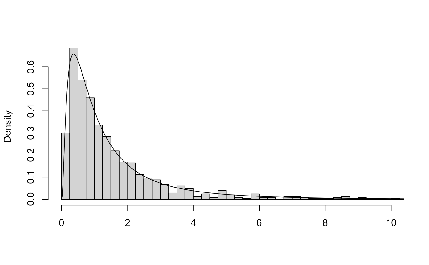
# Improve appearance using arguments to plot() and hist()
# \donttest{
plot(x, breaks = seq(0, ceiling(max(x$sim_vals)), by = 0.25),
  xlim = c(0, 10))

# }
# Two-dimensional normal with positive association ----------------
rho <- 0.9
covmat <- matrix(c(1, rho, rho, 1), 2, 2)
log_dmvnorm <- function(x, mean = rep(0, d), sigma = diag(d)) {
  x <- matrix(x, ncol = length(x))
  d <- ncol(x)
  - 0.5 * (x - mean) %*% solve(sigma) %*% t(x - mean)
}
x <- ru(logf = log_dmvnorm, sigma = covmat, d = 2, n = 1000, init = c(0, 0))
# \donttest{
plot(x)

# }

Plot diagnostics for an ru object

Usage

Arguments

Value

See also

Examples