Posterior predictive checks for a hef object

pp_check method for class "hef". This provides an interface to the functions that perform posterior predictive checks in the bayesplot package. See PPC-overview for details of these functions.

Usage

# S3 method for class 'hef'
pp_check(object, fun = NULL, raw = FALSE, nrep = NULL, ...)

Arguments

object: An object of class "hef", a result of a call to hef or hanova1.
fun: The plotting function to call. Can be any of the functions detailed at PPC-overview. The "ppc_" prefix can optionally be dropped if fun is specified as a string.
raw: Only relevant if object$model = "beta_binom" or object$model = "gamma_pois". If raw = TRUE then the raw responses are used in the plots. Otherwise, the proportions of successes are used in the beta_binom case and the exposure-adjusted rate in the gamma_pois case. In both cases the values used are object$data[, 1] / object$data[, 2] and the equivalent in object$data_rep.
nrep: The number of predictive replicates to use. If nrep is supplied then the first nrep rows of object$data_rep are used. Otherwise, or if nrep is greater than nrow(object$data_rep), then all rows are used.
...: Additional arguments passed on to bayesplot functions. See Examples below.

Value

A ggplot object that can be further customized using the ggplot2 package.

Details

For details of these functions see PPC-overview. See also the vignettes Conjugate Hierarchical Models, Hierarchical 1-way Analysis of Variance and the bayesplot vignette Graphical posterior predictive checks.

The general idea is to compare the observed data object$data with a matrix object$data_rep in which each row is a replication of the observed data simulated from the posterior predictive distribution. For greater detail see Chapter 6 of Gelman et al. (2013).

References

Jonah Gabry (2016). bayesplot: Plotting for Bayesian Models. R package version 1.1.0. https://CRAN.R-project.org/package=bayesplot

Gelman, A., Carlin, J. B., Stern, H. S., Dunson, D. B., Vehtari, A., and Rubin, D. B. (2013). Bayesian Data Analysis. Chapman & Hall/CRC Press, London, third edition. (Chapter 6). http://www.stat.columbia.edu/~gelman/book/

Examples

############################ Beta-binomial #################################

# ------------------------- Rat tumor data ------------------------------- #

rat_res <- hef(model = "beta_binom", data = rat, nrep = 50)

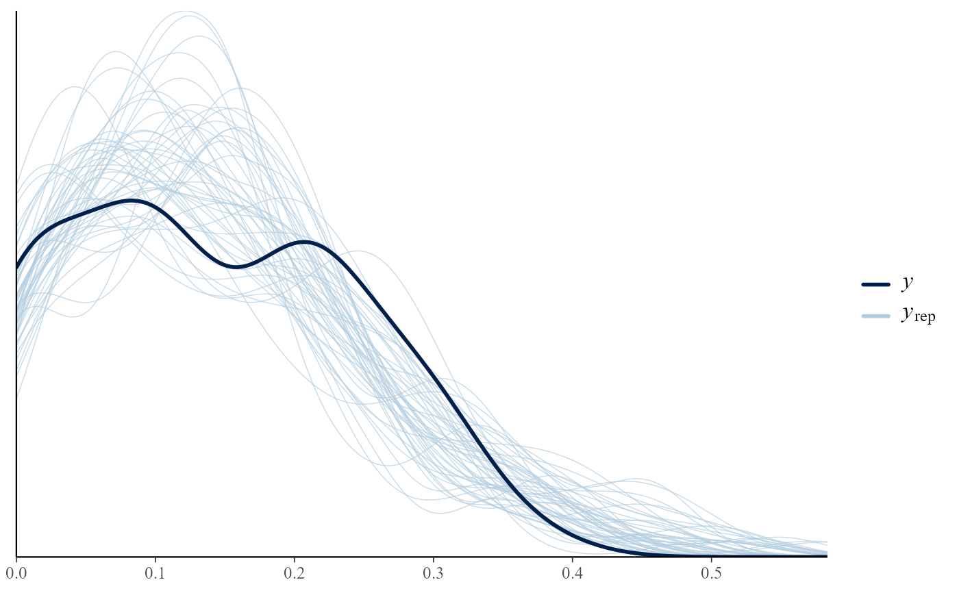
# Overlaid density estimates
pp_check(rat_res)

# \donttest{
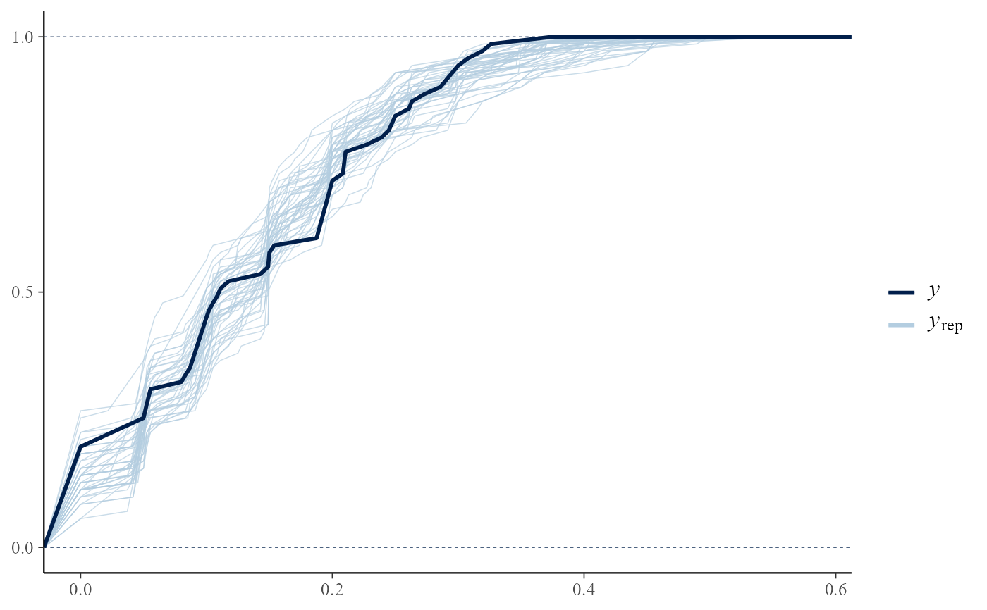
# Overlaid distribution function estimates
pp_check(rat_res, fun = "ecdf_overlay")

# }
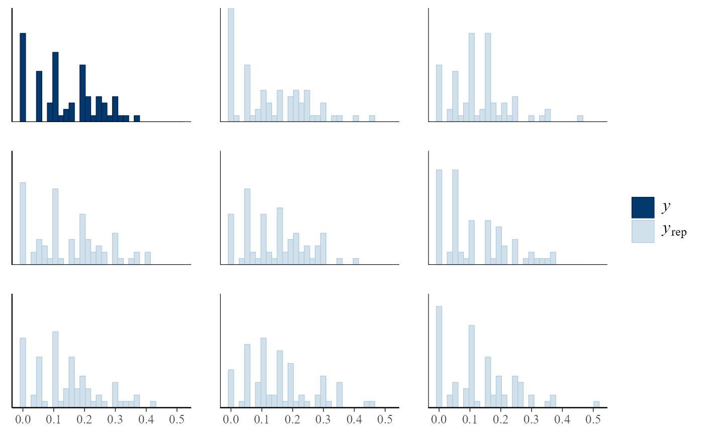
# Multiple histograms
pp_check(rat_res, fun = "hist", nrep = 8)
#> `stat_bin()` using `bins = 30`. Pick better value `binwidth`.

# \donttest{
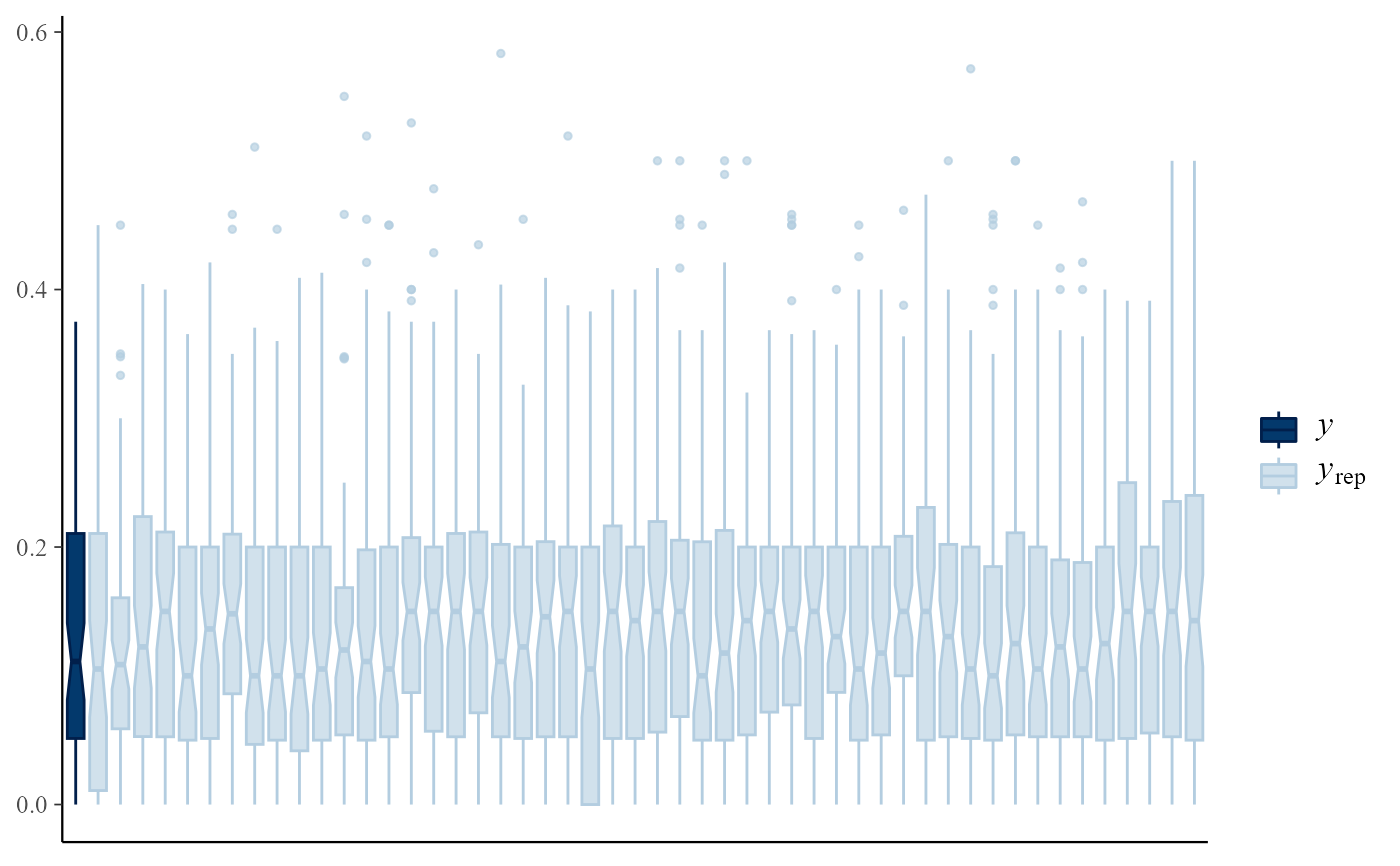
# Multiple boxplots
pp_check(rat_res, fun = "boxplot")

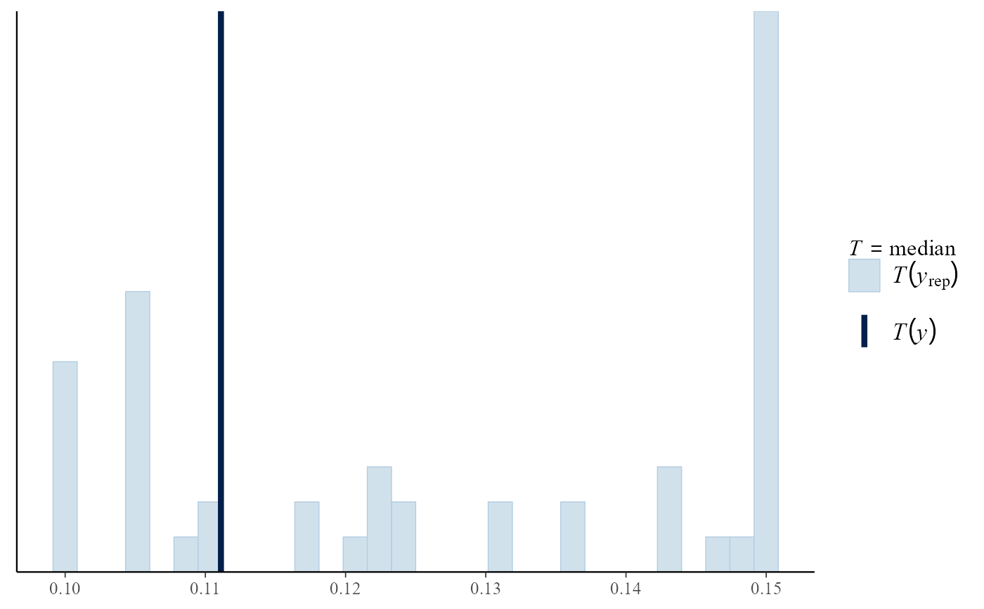
# Predictive medians vs observed median
pp_check(rat_res, fun = "stat", stat = "median")
#> `stat_bin()` using `bins = 30`. Pick better value `binwidth`.

# }
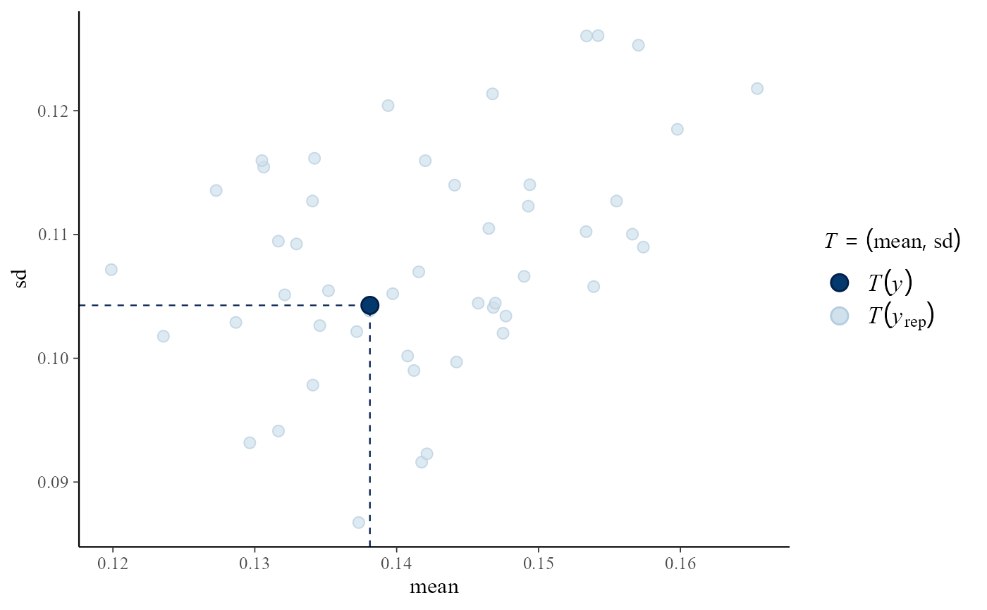
# Predictive (mean, sd) vs observed (mean, sd)
pp_check(rat_res, fun = "stat_2d", stat = c("mean", "sd"))
#> Note: in most cases the default test statistic 'mean' is too weak to detect anything of interest.


############################ Gamma-Poisson #################################

# ------------------------ Pump failure data ------------------------------ #

pump_res <- hef(model = "gamma_pois", data = pump, nrep = 50)

# \donttest{
# Overlaid density estimates
pp_check(pump_res)

# Predictive (mean, sd) vs observed (mean, sd)
pp_check(pump_res, fun = "stat_2d", stat = c("mean", "sd"))
#> Note: in most cases the default test statistic 'mean' is too weak to detect anything of interest.

# }

###################### One-way Hierarchical ANOVA ##########################

#----------------- Late 21st Century Global Temperature Data ------------- #

RCP26_2 <- temp2[temp2$RCP == "rcp26", ]
temp_res <- hanova1(resp = RCP26_2[, 1], fac = RCP26_2[, 2], nrep = 50)
# \donttest{
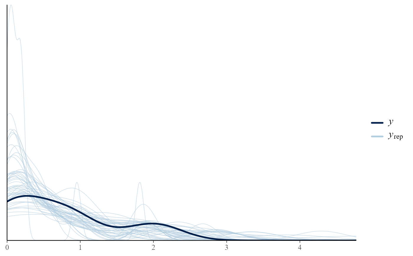
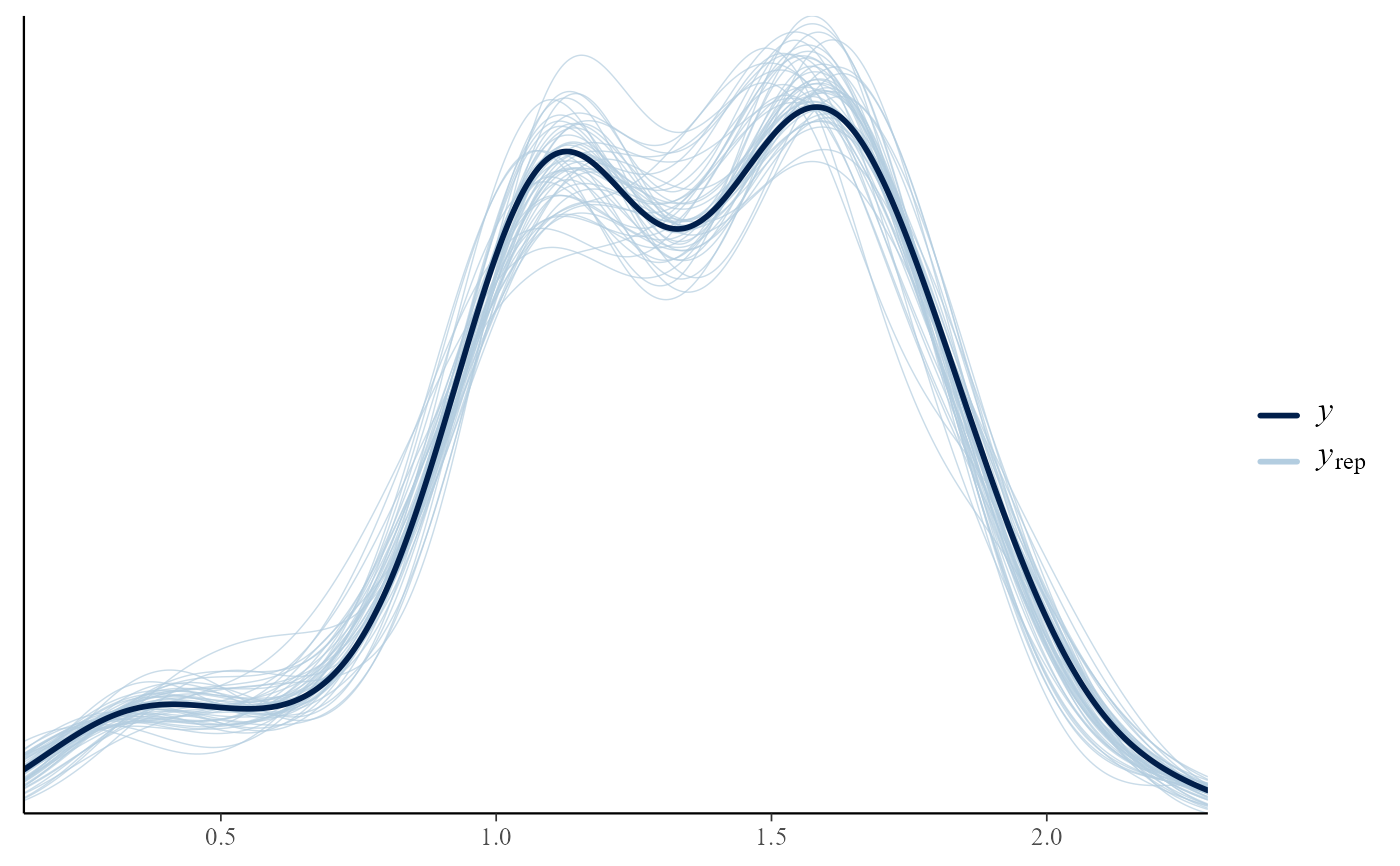
# Overlaid density estimates
pp_check(temp_res)

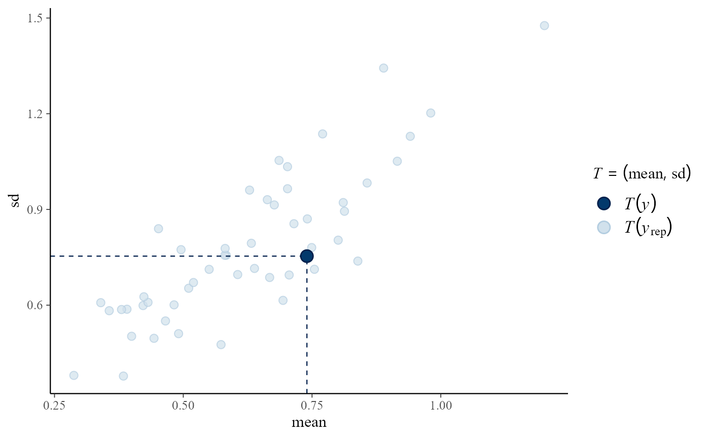
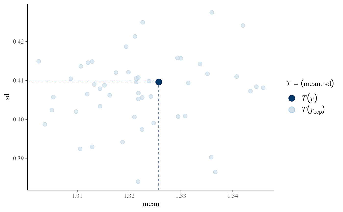
# Predictive (mean, sd) vs observed (mean, sd)
pp_check(temp_res, fun = "stat_2d", stat = c("mean", "sd"))
#> Note: in most cases the default test statistic 'mean' is too weak to detect anything of interest.

# }