GEV influence curves

Calculates influence function curves for maximum likelihood estimators of Generalised Extreme Value (GEV) parameters.

Usage

gev_influence(z, mu = 0, sigma = 1, xi = 0)

# S3 method for class 'gev_influence'
plot(x, xvar = c("z", "y"), sep_xi = TRUE, vlines, ...)

Arguments

z: A numeric vector. Values of normal quantiles \(z\) at which to calculate the GEV influence function. See Details.
mu, sigma, xi: Numeric scalars supplying the values of the GEV parameters \(\mu\), \(\sigma\) and \(\xi\).
x: An object inheriting from class "gev_influence", from a call to gev_influence.
xvar: A logical scalar. If xvar = "z" then the influence curves are plotted against the standard normal quantiles in x[, "z"]. If xvar = "y" then the influence curves are plotted against the corresponding GEV quantiles in x[, "y"].
sep_xi: A logical scalar. If sep_xi = TRUE then separate vertical scales are used for \(\xi\) and \((\mu, \sigma)\). The scale for \(\xi\) appears on the left and the scale for \((\mu, \sigma)\) on the right.
vlines: A numeric vector. If vlines is supplied then black dashed vertical lines are added to the plot at the values in vlines on the horizontal axis. This might be used to indicate the values of certain observations in a dataset.
...: For plot.gev_influence: to pass graphical parameters to the graphical functions matplot and legend. The parameters col, lty and lwd can be used to control line colour, type and width, with the parameters in the usual order, that is, \((\mu, \sigma, \xi)\).

Value

gev_influence: an object with class c("gev_influence", "matrix", "array"), a length(z) by 5 numeric matrix. The first two columns contain the input values in z and the corresponding values of y. Columns 3-5 contain the values of the GEV influence function for \(\mu\), \(\sigma\) and \(\xi\) respectively at the values of z.

plot.gev_influence: a list of the graphical parameters used in producing the plot, either the defaults or supplied via ..., is returned invisibly.

Details

An influence function measures the effect on a parameter estimator of changing one observation in a sample. See Hampel (2005) and, in the context of extreme value analyses of threshold exceedances, Davison and Smith (1990). Let \(\theta = (\mu, \sigma, \xi)\). The GEV influence curve is defined, as a function of an observation \(y\), by \(IC(y) = \{IC_{\mu}(y), IC_{\sigma}(y), IC_{\xi}(y)\} = i_\theta^{-1} {\rm d}\ell(y; \theta)/{\rm d} \theta\), where \(\ell(y; \theta)\) is the GEV log-likelihood function and \(i_\theta^{-1}\) is the GEV expected information matrix. The value of \(y\) is related to \(z\) by \(y = G^{-1}\{\Phi(z)\}\), where \(\Phi\) and \(G\) are the distribution functions of a standard normal and GEV(\(\mu, \sigma, \xi\)) distribution, respectively. Plotting influence curves on the standard normal z scale can help to aid interpretation.

The value of \(IC(y)\) is invariant to the value of \(\mu\). 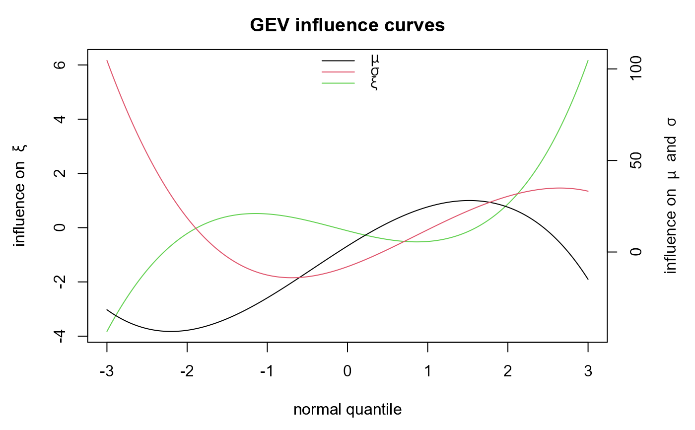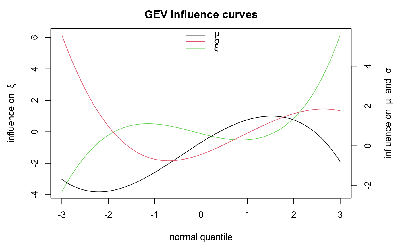For a given value of \(\xi\), the values of \(IC_{\mu}(y)\) and \(IC_{\sigma}(y)\) scale with the scale parameter \(\sigma\), that is, doubling \(\sigma\) doubles \(IC_{\mu}(y)\) and \(IC_{\sigma}(y).\) Typically, interest focuses on the shape parameter \(\xi\), but if the input scale parameter \(\sigma\) is large then this may hide the influence of \(y\) on \(\xi\). Therefore, the default setting of plot.gev_influence, sep_xi = TRUE, separates the plotting of the influence curve for \(\xi\) from those of \(\mu\) and \(\sigma\).

The example in Examples shows that extremely large block maxima have a strong positive influence on the MLE \(\hat{\xi}\) and also that extremely small block maxima have a strong negative influence on \(\hat{\xi}\),

References

Hampel, F. R., Ronchetti, E. M., Rousseeuw, P. J., and Stahel, W. A. (2005). Robust Statistics. Wiley-Interscience, New York. doi:10.1002/9781118186435

Davison, A. C. and Smith, R. L. (1990). Models for exceedances over high thresholds. Journal of the Royal Statistical Society: Series B (Methodological), 52(3):393–425. doi:10.1111/j.2517-6161.1990.tb01796.x

Examples

# Influence curve for the default mu = 0, sigma = 1, xi = 0 case
z <- seq(from = -3, to = 3, by = 0.01)
inf <- gev_influence(z = z)
plot(inf)


# Influence curves based on the adjusted fit to the Plymouth ozone data
fit <- gev_mle(PlymouthOzoneMaxima)
pars <- coef(fit)
infp <- gev_influence(z = z, mu = pars[1], sigma = pars[2], xi = pars[3])
plot(infp)