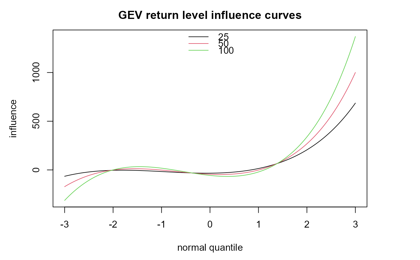
GEV influence curves for return levels

Calculates influence function curves for maximum likelihood estimators of 3 return levels based on Generalised Extreme Value (GEV) parameters.

Usage

gev_influence_rl(z, mu = 0, sigma = 1, xi = 0, m, npy = 1)

# S3 method for class 'gev_influence_rl'
plot(x, xvar = c("z", "y"), vlines, ...)

Arguments

z: A numeric vector. Values of normal quantiles \(z\) at which to calculate the GEV influence function. See Details.
mu, sigma, xi: Numeric scalars supplying the values of the GEV parameters \(\mu\), \(\sigma\) and \(\xi\).
m: A numeric vector of length 3 containing 3 unique return periods in years. All entries in m must be greater than 1.
npy: A numeric scalar. The number \(n_{py}\) of block maxima per year. If the blocks are of length 1 year then npy = 1.
x: An object inheriting from class "gev_influence_rl", returned from a call to gev_influence_rl.
xvar: A logical scalar. If xvar = "z" then the influence curves are plotted against the standard normal quantiles in x[, "z"]. If xvar = "y" then the influence curves are plotted against the corresponding GEV quantiles in x[, "y"].
vlines: A numeric vector. If vlines is supplied then black dashed vertical lines are added to the plot at the values in vlines on the horizontal axis. This might be used to indicate the values of certain observations in a dataset.
...: For plot.gev_influence_rl: to pass graphical parameters to the graphical functions matplot and legend. The parameters col, lty and lwd can be used to control line colour, type and width, with the return levels in the order that they were supplied in m.

Value

gev_influence_rl: an object with class c("gev_influence_rl", "matrix", "array"), a length(z) by 5 numeric matrix. The first two columns contain the input values in z and the corresponding values of y. Columns 3-5 contain the values of the GEV influence function for the return levels in m respectively at the values of z.

plot.gev_influence_rl: a list of the graphical parameters used in producing the plot, either the defaults or supplied via ..., is returned invisibly.

Details

See gev_influence for information about influence functions in general and influence curves for the parameters of a GEV distribution in particular. The GEV influence curves are reparameterised from \((\mu, \sigma, \xi)\) to the required return levels.

References

Hampel, F. R., Ronchetti, E. M., Rousseeuw, P. J., and Stahel, W. A. (2005). Robust Statistics. Wiley-Interscience, New York. doi:10.1002/9781118186435

Davison, A. C. and Smith, R. L. (1990). Models for exceedances over high thresholds. Journal of the Royal Statistical Society: Series B (Methodological), 52(3):393–425. doi:10.1111/j.2517-6161.1990.tb01796.x

Examples

# Influence curves based on the adjusted fit to the Plymouth ozone data
z <- seq(from = -3, to = 3, by = 0.01)
fit <- gev_mle(PlymouthOzoneMaxima)
pars <- coef(fit)
m <- c(25, 50, 100)
infp <- gev_influence_rl(z = z, mu = pars[1], sigma = pars[2], xi = pars[3],
                         m = m)
plot(infp)