Fits a Generalized Additive Model (GAM) for Location, Scale and Shape with
a GEV response distribution, using the function
gamlss::gamlss().
Usage
fitGEV(
  formula,
  data,
  scoring = c("fisher", "quasi"),
  mu.link = "identity",
  sigma.link = "log",
  xi.link = "identity",
  stepLength = 1,
  stepAttempts = 2,
  stepReduce = 2,
  steps = FALSE,
  ...
)
Arguments
- formula
a formula object, with the response on the left of an ~ operator, and the terms, separated by \(+\) operators, on the right. Nonparametric smoothing terms are indicated by
pb()for penalised beta splines,csfor smoothing splines,loforloesssmooth terms andrandomorrafor random terms, e.g.y~cs(x,df=5)+x1+x2*x3. Additional smoothers can be added by creating the appropriate interface. Interactions with nonparametric smooth terms are not fully supported, but will not produce errors; they will simply produce the usual parametric interaction- data
a data frame containing the variables occurring in the formula, e.g.
data=aids. If this is missing, the variables should be on the search list.- scoring
A character scalar. If
scoring = "fisher"then the weights used in the fitting algorithm are based on the expected Fisher information, that is, a Fisher's scoring algorithm is used. Ifscoring = "quasi"then these weights are based on the cross products of the first derivatives of the log-likelihood, leading to a quasi Newton scoring algorithm.- mu.link, sigma.link, xi.link
Character scalars to set the respective link functions for the location (
mu), scale (sigma) and shape (xi) parameters. The latter is passed togamlss::gamlss()asnu.link.- stepLength
A numeric vector of positive values. The initial values of the step lengths
mu.step,sigma.stepandnu.steppassed togamlss::gamlss.control()in the first attempt to fit the model by callinggamlss::gamlss(). IfstepLengthhas a length that is less than 3 thenstepLengthis recycled to have length 3.- stepAttempts
A non-negative integer. If the first call to
gamlss::gamlss()throws an error then we makestepAttemptsfurther attempts to fit the model, each time dividing by 2 the values ofmu.step,sigma.stepandnu.stepsupplied togamlss::gamlss.control(). IfstepAttempts < 1then no further attempts are made.- stepReduce
A number greater than 1. The factor by which the step lengths in
stepLengthare reduced for each extra attempt to fit the model. The default,stepReduce = 2means that the step lengths are halved for each extra attempt.- steps
A logical scalar. Pass
steps = TRUEto write to the console the current value ofstepLengthfor each call togamlss::gamlss().- ...
Further arguments passed to
gamlss::gamlss(), in particularmethod, which sets the fitting algorithm, with optionsRS(),CG()ormixed(). The default,method = RS()seems to work well, as doesmethod = mixed(). In contrast,method = CG()often requires the step length to be reduced before convergence is achieved.fitGEV()attempts to do this automatically. SeestepAttempts. Passtrace = FALSE(togamlss::gamlss.control()) to avoid writing to the console the global deviance after each outer iteration of the gamlss fitting algorithm.
Value
Returns a gamlss object. See the Value section of
gamlss::gamlss(). The class of the returned object is
c("gamlssx", "gamlss", "gam", "glm", "lm").
Details
See gamlss::gamlss() for information about
the model and the fitting algorithm.
Examples
# Load gamlss, for the functions term.plot() and wp()
library(gamlss)
#> Loading required package: splines
#> Loading required package: gamlss.data
#>
#> Attaching package: 'gamlss.data'
#> The following object is masked from 'package:datasets':
#>
#> sleep
#> Loading required package: gamlss.dist
#> Loading required package: nlme
#> Loading required package: parallel
#> ********** GAMLSS Version 5.5-0 **********
#> For more on GAMLSS look at https://www.gamlss.com/
#> Type gamlssNews() to see new features/changes/bug fixes.
##### Simulated data
set.seed(17012023)
n <- 100
x <- stats::runif(n)
mu <- 1 + 2 * x
sigma <- 1
xi <- 0.25
y <- nieve::rGEV(n = 1, loc = mu, scale = sigma, shape = xi)
data <- data.frame(y = as.numeric(y), x = x)
plot(x, y)
 # Fit model using the default RS method with Fisher's scoring
mod <- fitGEV(y ~ pb(x), data = data)
#> GAMLSS-RS iteration 1: Global Deviance = 323.1514
#> GAMLSS-RS iteration 2: Global Deviance = 320.4992
#> GAMLSS-RS iteration 3: Global Deviance = 320.1412
#> GAMLSS-RS iteration 4: Global Deviance = 320.091
#> GAMLSS-RS iteration 5: Global Deviance = 320.0839
#> GAMLSS-RS iteration 6: Global Deviance = 320.0829
# Summary of model fit
summary(mod)
#> ******************************************************************
#> Family: c("GEV", "Generalized Extreme Value")
#>
#> Call:
#> gamlss::gamlss(formula = y ~ pb(x), family = GEVfisher(mu.link = "identity",
#> sigma.link = "log", nu.link = "identity"), data = data,
#> mu.step = c(1, 1, 1)[1], sigma.step = c(1, 1, 1
#> )[2], nu.step = c(1, 1, 1)[3])
#>
#> Fitting method: RS()
#>
#> ------------------------------------------------------------------
#> Mu link function: identity
#> Mu Coefficients:
#> Estimate Std. Error t value Pr(>|t|)
#> (Intercept) 1.2726 0.1921 6.626 2.00e-09 ***
#> pb(x) 1.3830 0.3192 4.332 3.63e-05 ***
#> ---
#> Signif. codes: 0 '***' 0.001 '**' 0.01 '*' 0.05 '.' 0.1 ' ' 1
#>
#> ------------------------------------------------------------------
#> Sigma link function: log
#> Sigma Coefficients:
#> Estimate Std. Error t value Pr(>|t|)
#> (Intercept) -0.08761 0.09058 -0.967 0.336
#>
#> ------------------------------------------------------------------
#> Nu link function: identity
#> Nu Coefficients:
#> Estimate Std. Error t value Pr(>|t|)
#> (Intercept) 0.19264 0.08477 2.272 0.0253 *
#> ---
#> Signif. codes: 0 '***' 0.001 '**' 0.01 '*' 0.05 '.' 0.1 ' ' 1
#>
#> ------------------------------------------------------------------
#> NOTE: Additive smoothing terms exist in the formulas:
#> i) Std. Error for smoothers are for the linear effect only.
#> ii) Std. Error for the linear terms maybe are not accurate.
#> ------------------------------------------------------------------
#> No. of observations in the fit: 100
#> Degrees of Freedom for the fit: 4.000272
#> Residual Deg. of Freedom: 95.99973
#> at cycle: 6
#>
#> Global Deviance: 320.0829
#> AIC: 328.0835
#> SBC: 338.5049
#> ******************************************************************
# Residual diagnostic plots
plot(mod, xlab = "x", ylab = "y")
# Fit model using the default RS method with Fisher's scoring
mod <- fitGEV(y ~ pb(x), data = data)
#> GAMLSS-RS iteration 1: Global Deviance = 323.1514
#> GAMLSS-RS iteration 2: Global Deviance = 320.4992
#> GAMLSS-RS iteration 3: Global Deviance = 320.1412
#> GAMLSS-RS iteration 4: Global Deviance = 320.091
#> GAMLSS-RS iteration 5: Global Deviance = 320.0839
#> GAMLSS-RS iteration 6: Global Deviance = 320.0829
# Summary of model fit
summary(mod)
#> ******************************************************************
#> Family: c("GEV", "Generalized Extreme Value")
#>
#> Call:
#> gamlss::gamlss(formula = y ~ pb(x), family = GEVfisher(mu.link = "identity",
#> sigma.link = "log", nu.link = "identity"), data = data,
#> mu.step = c(1, 1, 1)[1], sigma.step = c(1, 1, 1
#> )[2], nu.step = c(1, 1, 1)[3])
#>
#> Fitting method: RS()
#>
#> ------------------------------------------------------------------
#> Mu link function: identity
#> Mu Coefficients:
#> Estimate Std. Error t value Pr(>|t|)
#> (Intercept) 1.2726 0.1921 6.626 2.00e-09 ***
#> pb(x) 1.3830 0.3192 4.332 3.63e-05 ***
#> ---
#> Signif. codes: 0 '***' 0.001 '**' 0.01 '*' 0.05 '.' 0.1 ' ' 1
#>
#> ------------------------------------------------------------------
#> Sigma link function: log
#> Sigma Coefficients:
#> Estimate Std. Error t value Pr(>|t|)
#> (Intercept) -0.08761 0.09058 -0.967 0.336
#>
#> ------------------------------------------------------------------
#> Nu link function: identity
#> Nu Coefficients:
#> Estimate Std. Error t value Pr(>|t|)
#> (Intercept) 0.19264 0.08477 2.272 0.0253 *
#> ---
#> Signif. codes: 0 '***' 0.001 '**' 0.01 '*' 0.05 '.' 0.1 ' ' 1
#>
#> ------------------------------------------------------------------
#> NOTE: Additive smoothing terms exist in the formulas:
#> i) Std. Error for smoothers are for the linear effect only.
#> ii) Std. Error for the linear terms maybe are not accurate.
#> ------------------------------------------------------------------
#> No. of observations in the fit: 100
#> Degrees of Freedom for the fit: 4.000272
#> Residual Deg. of Freedom: 95.99973
#> at cycle: 6
#>
#> Global Deviance: 320.0829
#> AIC: 328.0835
#> SBC: 338.5049
#> ******************************************************************
# Residual diagnostic plots
plot(mod, xlab = "x", ylab = "y")
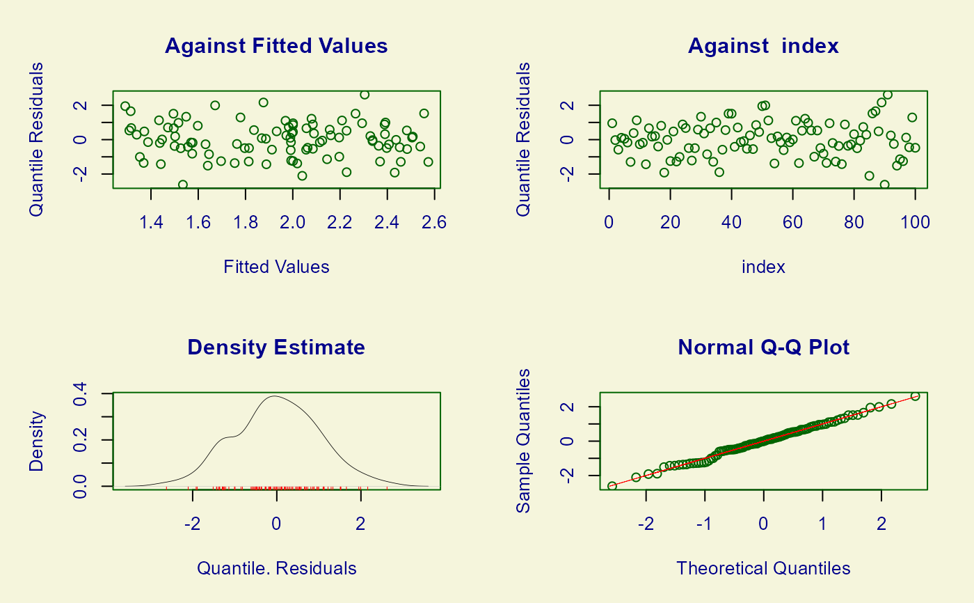 #> ******************************************************************
#> Summary of the Quantile Residuals
#> mean = -0.0005858247
#> variance = 1.00992
#> coef. of skewness = -0.007497414
#> coef. of kurtosis = 2.780556
#> Filliben correlation coefficient = 0.9973717
#> ******************************************************************
# Data plus fitted curve
plot(data$x, data$y, xlab = "x", ylab = "y")
lines(data$x, fitted(mod))
#> ******************************************************************
#> Summary of the Quantile Residuals
#> mean = -0.0005858247
#> variance = 1.00992
#> coef. of skewness = -0.007497414
#> coef. of kurtosis = 2.780556
#> Filliben correlation coefficient = 0.9973717
#> ******************************************************************
# Data plus fitted curve
plot(data$x, data$y, xlab = "x", ylab = "y")
lines(data$x, fitted(mod))
 # Fit model using the mixed method and quasi-Newton scoring
# Use trace = FALSE to prevent writing the global deviance to the console
mod <- fitGEV(y ~ pb(x), data = data, method = mixed(), scoring = "quasi",
trace = FALSE)
# Fit model using the CG method
# The default step length of 1 needs to be reduced to enable convergence
# Use steps = TRUE to write the step lengths to the console
mod <- fitGEV(y ~ pb(x), data = data, method = CG(), steps = TRUE)
#> stepLength = 1 1 1
#> stepLength = 0.5 0.5 0.5
#> GAMLSS-CG iteration 1: Global Deviance = 337.4163
#> GAMLSS-CG iteration 2: Global Deviance = 322.5637
#> GAMLSS-CG iteration 3: Global Deviance = 321.03
#> GAMLSS-CG iteration 4: Global Deviance = 320.4416
#> GAMLSS-CG iteration 5: Global Deviance = 320.2167
#> GAMLSS-CG iteration 6: Global Deviance = 320.1324
#> GAMLSS-CG iteration 7: Global Deviance = 320.1011
#> GAMLSS-CG iteration 8: Global Deviance = 320.0896
#> GAMLSS-CG iteration 9: Global Deviance = 320.0855
#> GAMLSS-CG iteration 10: Global Deviance = 320.0839
#> GAMLSS-CG iteration 11: Global Deviance = 320.0834
##### Fremantle annual maximum sea levels
##### See also the gamlssx package README file
# Transform Year so that it is centred on 0
fremantle <- transform(fremantle, cYear = Year - median(Year))
# Plot sea level against year and against SOI
plot(fremantle$Year, fremantle$SeaLevel, xlab = "year", ylab = "sea level (m)")
# Fit model using the mixed method and quasi-Newton scoring
# Use trace = FALSE to prevent writing the global deviance to the console
mod <- fitGEV(y ~ pb(x), data = data, method = mixed(), scoring = "quasi",
trace = FALSE)
# Fit model using the CG method
# The default step length of 1 needs to be reduced to enable convergence
# Use steps = TRUE to write the step lengths to the console
mod <- fitGEV(y ~ pb(x), data = data, method = CG(), steps = TRUE)
#> stepLength = 1 1 1
#> stepLength = 0.5 0.5 0.5
#> GAMLSS-CG iteration 1: Global Deviance = 337.4163
#> GAMLSS-CG iteration 2: Global Deviance = 322.5637
#> GAMLSS-CG iteration 3: Global Deviance = 321.03
#> GAMLSS-CG iteration 4: Global Deviance = 320.4416
#> GAMLSS-CG iteration 5: Global Deviance = 320.2167
#> GAMLSS-CG iteration 6: Global Deviance = 320.1324
#> GAMLSS-CG iteration 7: Global Deviance = 320.1011
#> GAMLSS-CG iteration 8: Global Deviance = 320.0896
#> GAMLSS-CG iteration 9: Global Deviance = 320.0855
#> GAMLSS-CG iteration 10: Global Deviance = 320.0839
#> GAMLSS-CG iteration 11: Global Deviance = 320.0834
##### Fremantle annual maximum sea levels
##### See also the gamlssx package README file
# Transform Year so that it is centred on 0
fremantle <- transform(fremantle, cYear = Year - median(Year))
# Plot sea level against year and against SOI
plot(fremantle$Year, fremantle$SeaLevel, xlab = "year", ylab = "sea level (m)")
 plot(fremantle$SOI, fremantle$SeaLevel, xlab = "SOI", ylab = "sea level (m)")
 # Fit a model with P-spline effects of cYear and SOI on location and scale
# The default links are identity for location and log for scale
mod <- fitGEV(SeaLevel ~ pb(cYear) + pb(SOI),
sigma.formula = ~ pb(cYear) + pb(SOI),
data = fremantle)
#> Error in fitGEV(SeaLevel ~ pb(cYear) + pb(SOI), sigma.formula = ~pb(cYear) + pb(SOI), data = fremantle): No convergence. An error was thrown from the last call to gamlss()
# Summary of model fit
summary(mod)
#> ******************************************************************
#> Family: c("GEV", "Generalized Extreme Value")
#>
#> Call:
#> gamlss::gamlss(formula = y ~ pb(x), family = GEVfisher(mu.link = "identity",
#> sigma.link = "log", nu.link = "identity"), data = data,
#> method = CG(), mu.step = c(0.5, 0.5, 0.5)[1], sigma.step = c(0.5,
#> 0.5, 0.5)[2], nu.step = c(0.5, 0.5, 0.5)[3])
#>
#> Fitting method: CG()
#>
#> ------------------------------------------------------------------
#> Mu link function: identity
#> Mu Coefficients:
#> Estimate Std. Error t value Pr(>|t|)
#> (Intercept) 1.2746 0.1923 6.628 1.99e-09 ***
#> pb(x) 1.3801 0.3198 4.315 3.88e-05 ***
#> ---
#> Signif. codes: 0 '***' 0.001 '**' 0.01 '*' 0.05 '.' 0.1 ' ' 1
#>
#> ------------------------------------------------------------------
#> Sigma link function: log
#> Sigma Coefficients:
#> Estimate Std. Error t value Pr(>|t|)
#> (Intercept) -0.08693 0.09060 -0.959 0.34
#>
#> ------------------------------------------------------------------
#> Nu link function: identity
#> Nu Coefficients:
#> Estimate Std. Error t value Pr(>|t|)
#> (Intercept) 0.19171 0.08467 2.264 0.0258 *
#> ---
#> Signif. codes: 0 '***' 0.001 '**' 0.01 '*' 0.05 '.' 0.1 ' ' 1
#>
#> ------------------------------------------------------------------
#> NOTE: Additive smoothing terms exist in the formulas:
#> i) Std. Error for smoothers are for the linear effect only.
#> ii) Std. Error for the linear terms maybe are not accurate.
#> ------------------------------------------------------------------
#> No. of observations in the fit: 100
#> Degrees of Freedom for the fit: 4.000271
#> Residual Deg. of Freedom: 95.99973
#> at cycle: 11
#>
#> Global Deviance: 320.0834
#> AIC: 328.0839
#> SBC: 338.5053
#> ******************************************************************
# Model diagnostic plots
plot(mod)
# Fit a model with P-spline effects of cYear and SOI on location and scale
# The default links are identity for location and log for scale
mod <- fitGEV(SeaLevel ~ pb(cYear) + pb(SOI),
sigma.formula = ~ pb(cYear) + pb(SOI),
data = fremantle)
#> Error in fitGEV(SeaLevel ~ pb(cYear) + pb(SOI), sigma.formula = ~pb(cYear) + pb(SOI), data = fremantle): No convergence. An error was thrown from the last call to gamlss()
# Summary of model fit
summary(mod)
#> ******************************************************************
#> Family: c("GEV", "Generalized Extreme Value")
#>
#> Call:
#> gamlss::gamlss(formula = y ~ pb(x), family = GEVfisher(mu.link = "identity",
#> sigma.link = "log", nu.link = "identity"), data = data,
#> method = CG(), mu.step = c(0.5, 0.5, 0.5)[1], sigma.step = c(0.5,
#> 0.5, 0.5)[2], nu.step = c(0.5, 0.5, 0.5)[3])
#>
#> Fitting method: CG()
#>
#> ------------------------------------------------------------------
#> Mu link function: identity
#> Mu Coefficients:
#> Estimate Std. Error t value Pr(>|t|)
#> (Intercept) 1.2746 0.1923 6.628 1.99e-09 ***
#> pb(x) 1.3801 0.3198 4.315 3.88e-05 ***
#> ---
#> Signif. codes: 0 '***' 0.001 '**' 0.01 '*' 0.05 '.' 0.1 ' ' 1
#>
#> ------------------------------------------------------------------
#> Sigma link function: log
#> Sigma Coefficients:
#> Estimate Std. Error t value Pr(>|t|)
#> (Intercept) -0.08693 0.09060 -0.959 0.34
#>
#> ------------------------------------------------------------------
#> Nu link function: identity
#> Nu Coefficients:
#> Estimate Std. Error t value Pr(>|t|)
#> (Intercept) 0.19171 0.08467 2.264 0.0258 *
#> ---
#> Signif. codes: 0 '***' 0.001 '**' 0.01 '*' 0.05 '.' 0.1 ' ' 1
#>
#> ------------------------------------------------------------------
#> NOTE: Additive smoothing terms exist in the formulas:
#> i) Std. Error for smoothers are for the linear effect only.
#> ii) Std. Error for the linear terms maybe are not accurate.
#> ------------------------------------------------------------------
#> No. of observations in the fit: 100
#> Degrees of Freedom for the fit: 4.000271
#> Residual Deg. of Freedom: 95.99973
#> at cycle: 11
#>
#> Global Deviance: 320.0834
#> AIC: 328.0839
#> SBC: 338.5053
#> ******************************************************************
# Model diagnostic plots
plot(mod)
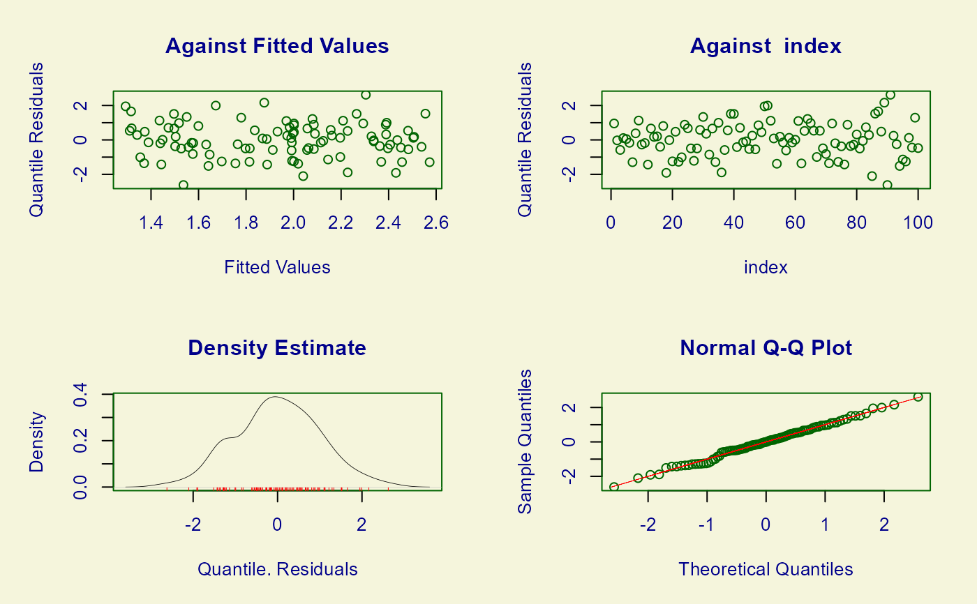 #> ******************************************************************
#> Summary of the Quantile Residuals
#> mean = -0.0006504536
#> variance = 1.009723
#> coef. of skewness = -0.004767227
#> coef. of kurtosis = 2.781026
#> Filliben correlation coefficient = 0.99738
#> ******************************************************************
# Worm plot
wp(mod)
#> Error in as.environment(DaTa): invalid object for 'as.environment'
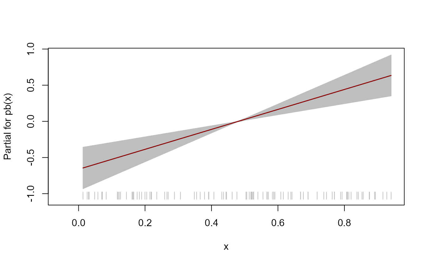
# Plot of the fitted component smooth functions
# Note: gamlss::term.plot() does not include uncertainty about the intercept
# Location mu
term.plot(mod, rug = TRUE, pages = 1)
#> ******************************************************************
#> Summary of the Quantile Residuals
#> mean = -0.0006504536
#> variance = 1.009723
#> coef. of skewness = -0.004767227
#> coef. of kurtosis = 2.781026
#> Filliben correlation coefficient = 0.99738
#> ******************************************************************
# Worm plot
wp(mod)
#> Error in as.environment(DaTa): invalid object for 'as.environment'
# Plot of the fitted component smooth functions
# Note: gamlss::term.plot() does not include uncertainty about the intercept
# Location mu
term.plot(mod, rug = TRUE, pages = 1)
 # Scale sigma
term.plot(mod, what = "sigma", rug = TRUE, pages = 1)
#> Error in term.plot(mod, what = "sigma", rug = TRUE, pages = 1): The model for sigma has only the constant fitted
# Scale sigma
term.plot(mod, what = "sigma", rug = TRUE, pages = 1)
#> Error in term.plot(mod, what = "sigma", rug = TRUE, pages = 1): The model for sigma has only the constant fitted