Frequentist threshold-based inference for return levels

Calculates point estimates and confidence intervals for m-year return levels for stationary time series fitted extreme value model objects returned from flite. Two types of interval may be returned: (a) intervals based on approximate large-sample normality of the maximum likelihood estimator for return level, which are symmetric about the point estimate, and (b) profile likelihood-based intervals based on an (adjusted) log-likelihood.

returnLevel(
  x,
  m = 100,
  level = 0.95,
  ny,
  prof = TRUE,
  inc = 1/100,
  type = c("vertical", "cholesky", "spectral", "none")
)

Arguments

x: An object inheriting from class "flite" returned from flite.
m: A numeric scalar. The return period, in years.
level: A numeric scalar in (0, 1). The confidence level required for confidence interval for the m-year return level.
ny: A numeric scalar. The (mean) number of observations per year. Setting this appropriately is important. See Details.
prof: A logical scalar. Should we calculate intervals based on profile log-likelihood?
inc: A numeric scalar in (0, 1/2]. Only relevant if prof = TRUE. The increment, a fraction of the length of the symmetric confidence interval for the m-year return level, by which we move upwards and downwards from the MLE for the return level in the search for the lower and upper confidence limits.
type: A character scalar. The argument type to the function returned by the function adjust_loglik, that is, the type of adjustment made to the independence log-likelihood function in creating an adjusted log-likelihood function. See Details and Value in adjust_loglik.

Value

A object (a list) of class "returnLevel", "lite" with the components

rl_sym,rl_prof: Named numeric vectors containing the respective lower 100level% limit, the MLE and the upper 100level% limit for the return level. If prof = FALSE then rl_prof will be missing.
rl_se: Estimated standard error of the return level.
max_loglik,crit,for_plot: If prof = TRUE then these components will be present, containing respectively: the maximised log-likelihood; the critical value and a matrix with return levels in the first column (ret_levs) and the corresponding values of the (adjusted) profile log-likelihood (prof_loglik).
m,level: The input values of m and level.
ny: The value of ny used to infer the return level.
call: The call to returnLevel.

Details

For information about return levels see the "Introducing lite" vignette.

ny provides information about the (intended) frequency of sampling in time, that is, the number of observations that would be observed in a year if there are no missing values. If the number of observations may vary between years then ny should be set equal to the mean number of observations per year.

Supplying ny. The value of ny may have been set in the call to flite. If ny is supplied by the user in the call to returnLevel then this will be used in preference to the value stored in the fitted model object. If these two values differ then no warning will be given.

For details of the definition and estimation of return levels see the Inference for return levels vignette.

The profile likelihood-based intervals are calculated by reparameterising in terms of the m-year return level and estimating the values at which the (adjusted) profile log-likelihood reaches the critical value logLik(x) - 0.5 * stats::qchisq(level, 1). This is achieved by calculating the profile log-likelihood for a sequence of values of this return level as governed by inc. Once the profile log-likelihood drops below the critical value the lower and upper limits are estimated by interpolating linearly between the cases lying either side of the critical value. The smaller inc the more accurate (but slower) the calculation will be.

References

Coles, S. G. (2001) An Introduction to Statistical Modeling of Extreme Values, Springer-Verlag, London. doi:10.1007/978-1-4471-3675-0_3

Examples

### Cheeseboro wind gusts

# Make inferences
cdata <- exdex::cheeseboro
# Each column of the matrix cdata corresponds to data from a different year
# flite() sets cluster automatically to correspond to column (year)
cfit <- flite(cdata, u = 45, k = 3)

# These data are hourly for one month (January) year so ny = 31 * 24
# Large inc set here for speed, sacrificing accuracy
# Default 95% confidence intervals
rl <- returnLevel(cfit, inc = 1 / 10, ny = 31 * 24)
summary(rl)
#> 
#> Call:
#> returnLevel(x = cfit, ny = 31 * 24, inc = 1/10)
#> 
#>         Estimate Std. Error
#> m = 100 88.61986   9.600889
rl
#> 
#> Call:
#> returnLevel(x = cfit, ny = 31 * 24, inc = 1/10)
#> 
#> MLE and 95% confidence limits for the 100-year return level
#> 
#> Normal interval:
#>  lower     mle   upper  
#>  69.80   88.62  107.44  
#> Profile likelihood-based interval:
#>  lower     mle   upper  
#>  76.15   88.62  125.45  
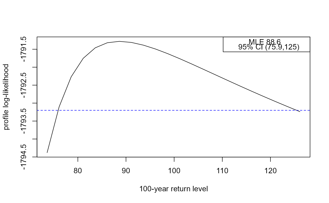
oldrl <- plot(rl)

oldrl
#>     lower       mle     upper 
#>  76.15487  88.61986 125.44775 

# Quickly recalculate/replot the intervals based on profile log-likelihood
# provided that level is smaller than that used to produce rl
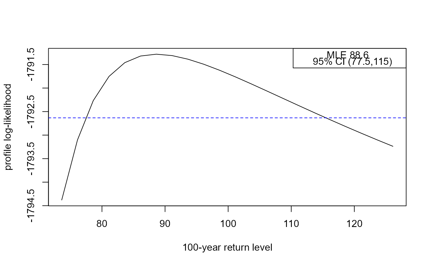
newrl <- plot(rl, level = 0.9)

newrl
#>     lower       mle     upper 
#>  77.40536  88.61986 115.49662