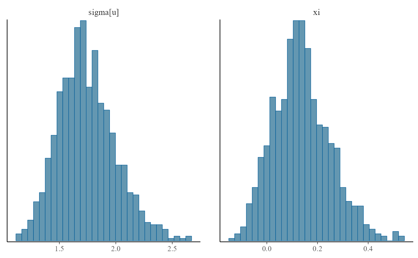
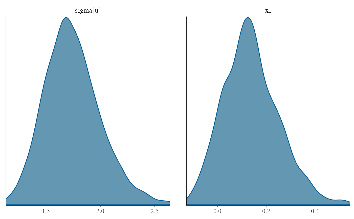
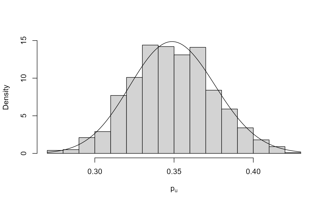
Plot diagnostics for an evpost object

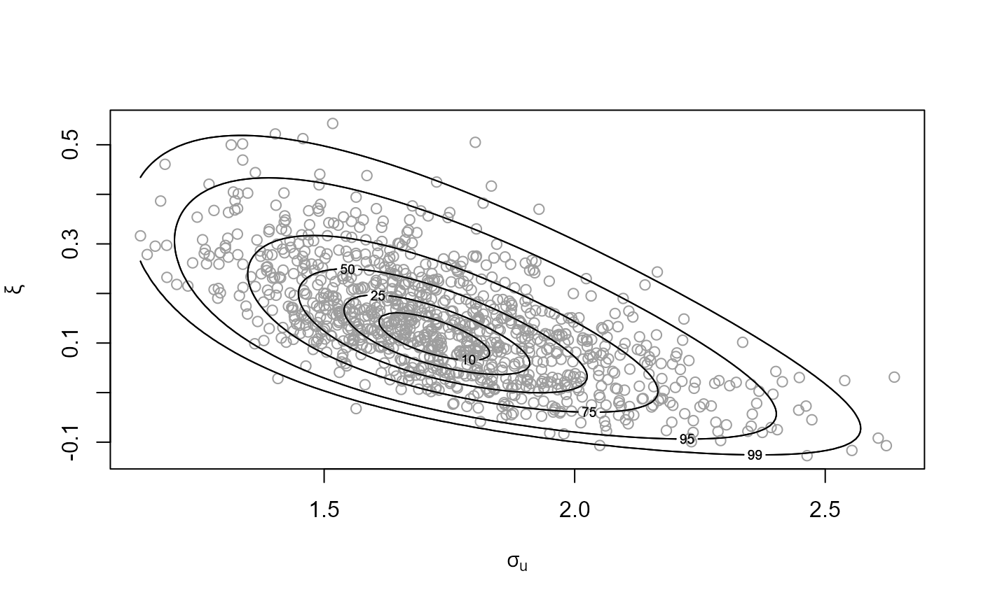
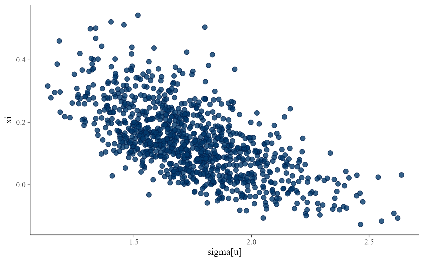
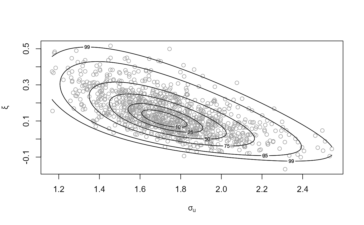
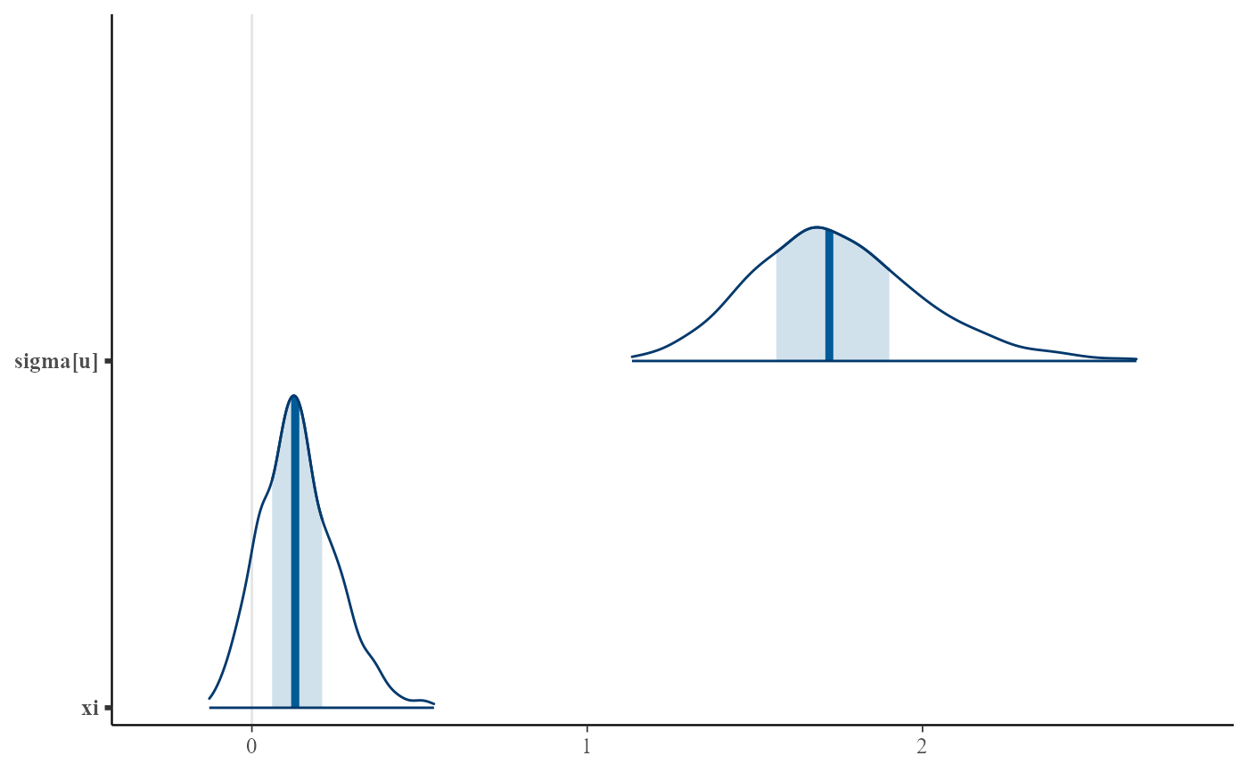
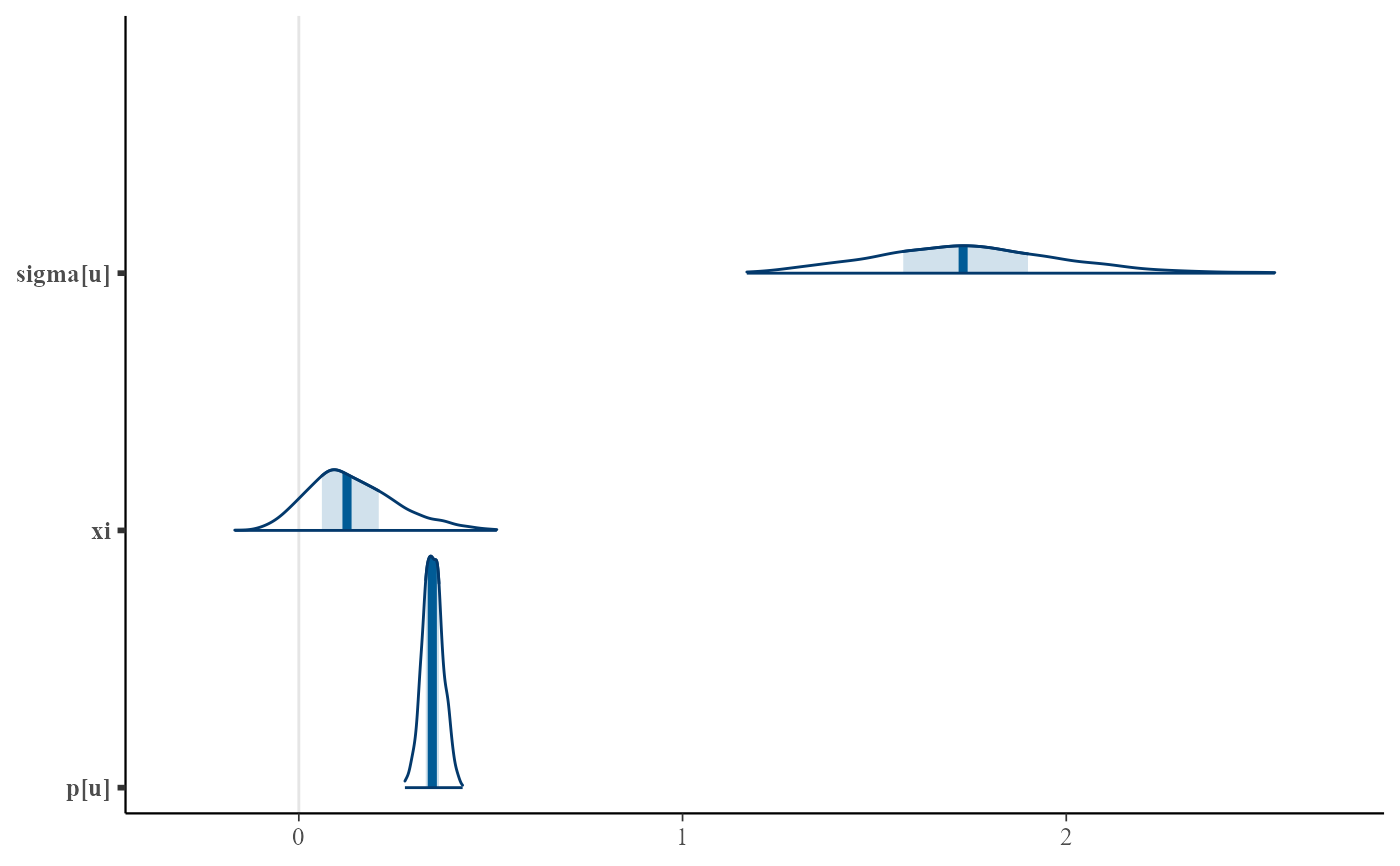
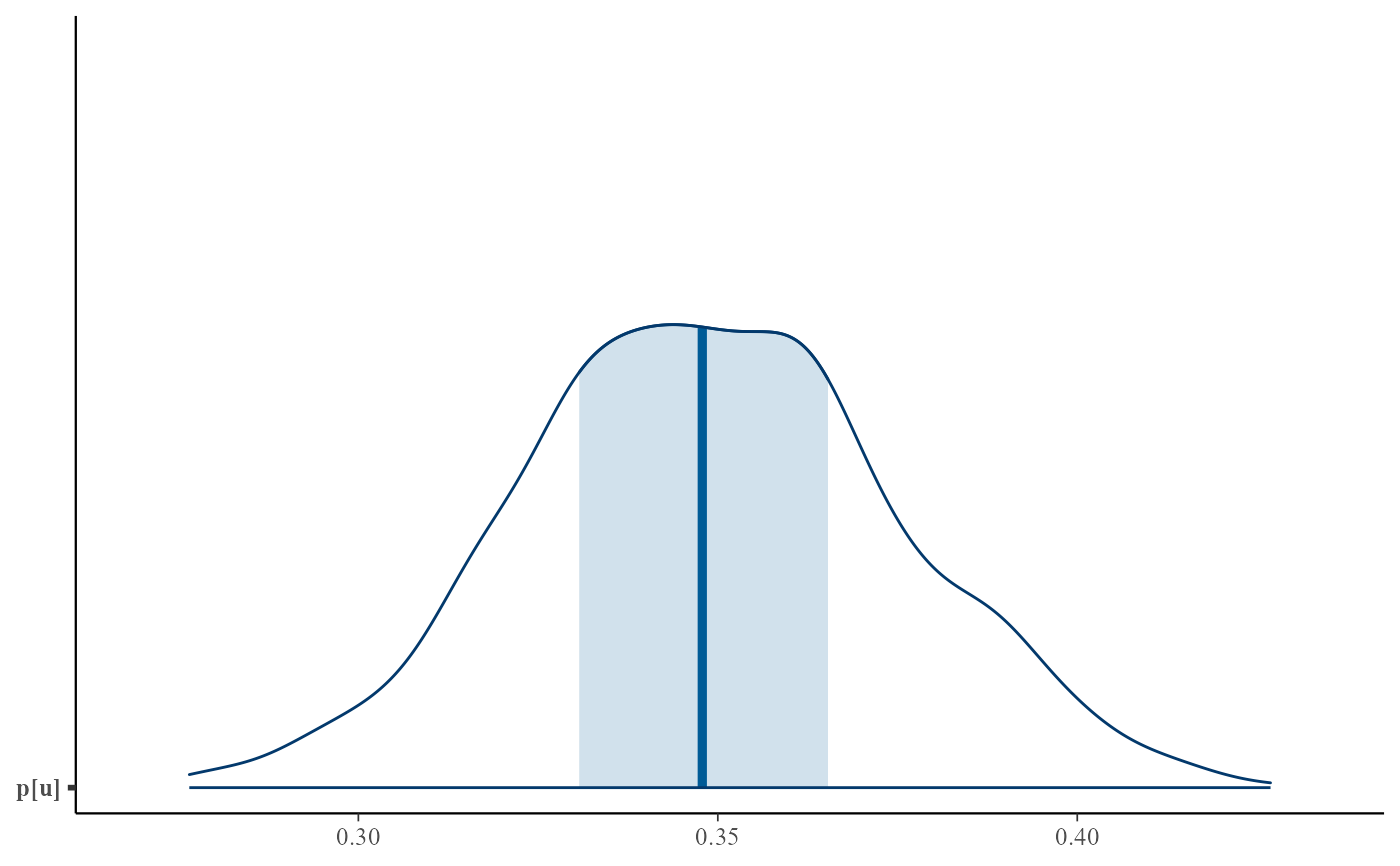
plot method for class "evpost". For d = 1 a histogram of the simulated values is plotted with a the density function superimposed. The density is normalized crudely using the trapezium rule. For d = 2 a scatter plot of the simulated values is produced with density contours superimposed. For d > 2 pairwise plots of the simulated values are produced. An interface is also provided to the functions in the bayesplot package that produce plots of Markov chain Monte Carlo (MCMC) simulations. See MCMC-overview for details of these functions.

Usage

# S3 method for class 'evpost'
plot(
  x,
  y,
  ...,
  n = ifelse(x$d == 1, 1001, 101),
  prob = c(0.5, 0.1, 0.25, 0.75, 0.95, 0.99),
  ru_scale = FALSE,
  rows = NULL,
  xlabs = NULL,
  ylabs = NULL,
  points_par = list(col = 8),
  pu_only = FALSE,
  add_pu = FALSE,
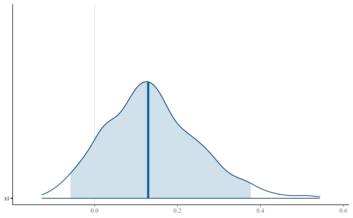
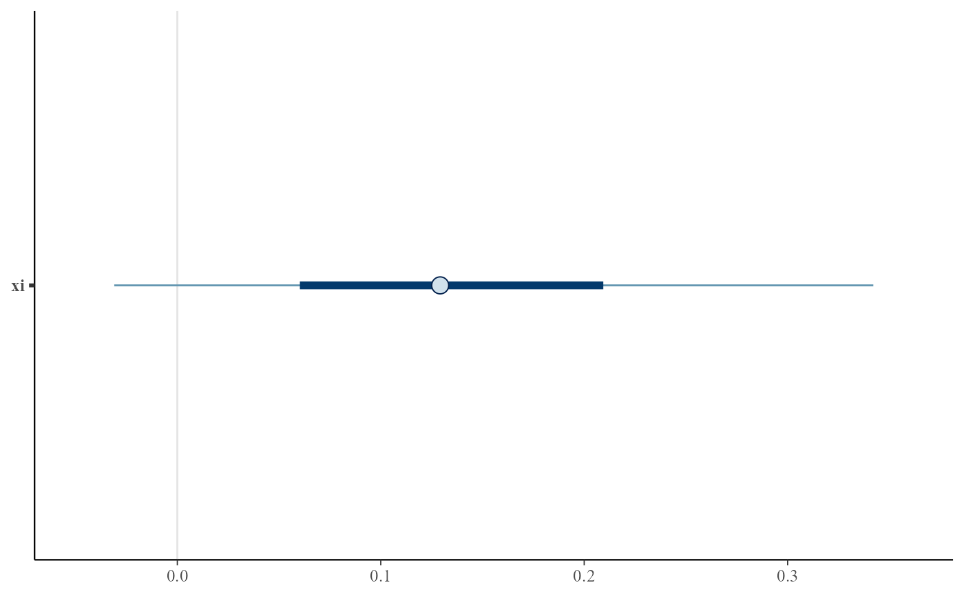
  use_bayesplot = FALSE,
  fun_name = c("areas", "intervals", "dens", "hist", "scatter")
)

Arguments

x

An object of class "evpost", a result of a call to rpost or rpost_rcpp.

y

Not used.

...

Additional arguments passed on to hist, lines, contour, points or functions from the bayesplot package.

n

A numeric scalar. Only relevant if x$d = 1 or x$d = 2. The meaning depends on the value of x$d.

For d = 1 : n + 1 is the number of abscissae in the trapezium method used to normalize the density.
For d = 2 : an n by n regular grid is used to contour the density.

prob

Numeric vector. Only relevant for d = 2. The contour lines are drawn such that the respective probabilities that the variable lies within the contour are approximately prob.

ru_scale

A logical scalar. Should we plot data and density on the scale used in the ratio-of-uniforms algorithm (TRUE) or on the original scale (FALSE)?

rows

A numeric scalar. When d > 2 this sets the number of rows of plots. If the user doesn't provide this then it is set internally.

xlabs, ylabs

Numeric vectors. When d > 2 these set the labels on the x and y axes respectively. If the user doesn't provide these then the column names of the simulated data matrix to be plotted are used.

points_par

A list of arguments to pass to points to control the appearance of points depicting the simulated values. Only relevant when d = 2.

pu_only

Only produce a plot relating to the posterior distribution for the threshold exceedance probability $p$. Only relevant when model == "bingp" was used in the call to rpost or rpost_rcpp.

add_pu

Before producing the plots add the threshold exceedance probability $p$ to the parameters of the extreme value model. Only relevant when model == "bingp" was used in the call to rpost or rpost_rcpp.

use_bayesplot

A logical scalar. If TRUE the bayesplot function indicated by fun_name is called. In principle any bayesplot function (that starts with mcmc_) can be called but this may not always be successful because, for example, some of the bayesplot functions work only with multiple MCMC simulations.

fun_name

A character scalar. The name of the bayesplot function, with the initial mcmc_ part removed. See MCMC-overview and links therein for the names of these functions. Some examples are given below.

Value

Nothing is returned unless use_bayesplot = TRUE when a ggplot object, which can be further customized using the ggplot2 package, is returned.

Details

For details of the bayesplot functions available when use_bayesplot = TRUE see MCMC-overview and the bayesplot vignette Plotting MCMC draws.

References

Jonah Gabry (2016). bayesplot: Plotting for Bayesian Models. R package version 1.1.0. https://CRAN.R-project.org/package=bayesplot

Examples

## GP posterior
u <- stats::quantile(gom, probs = 0.65)
fp <- set_prior(prior = "flat", model = "gp", min_xi = -1)
gpg <- rpost(n = 1000, model = "gp", prior = fp, thresh = u, data = gom)
plot(gpg)


# \donttest{
# Using the bayesplot package
plot(gpg, use_bayesplot = TRUE)

plot(gpg, use_bayesplot = TRUE, pars = "xi", prob = 0.95)

plot(gpg, use_bayesplot = TRUE, fun_name = "intervals", pars = "xi")

plot(gpg, use_bayesplot = TRUE, fun_name = "hist")
#> `stat_bin()` using `bins = 30`. Pick better value `binwidth`.

plot(gpg, use_bayesplot = TRUE, fun_name = "dens")

plot(gpg, use_bayesplot = TRUE, fun_name = "scatter")

# }

## bin-GP posterior
u <- quantile(gom, probs = 0.65)
fp <- set_prior(prior = "flat", model = "gp", min_xi = -1)
bp <- set_bin_prior(prior = "jeffreys")
npy_gom <- length(gom)/105
bgpg <- rpost(n = 1000, model = "bingp", prior = fp, thresh = u,
              data = gom, bin_prior = bp, npy = npy_gom)
plot(bgpg)

plot(bgpg, pu_only = TRUE)

plot(bgpg, add_pu = TRUE)


# \donttest{
# Using the bayesplot package
dimnames(bgpg$bin_sim_vals)
#> [[1]]
#> NULL
#> 
#> [[2]]
#> [1] "p[u]"
#> 
plot(bgpg, use_bayesplot = TRUE)

plot(bgpg, use_bayesplot = TRUE, fun_name = "hist")
#> `stat_bin()` using `bins = 30`. Pick better value `binwidth`.

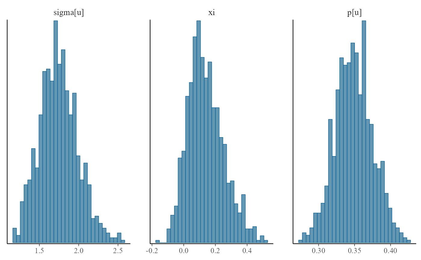plot(bgpg, use_bayesplot = TRUE, pars = "p[u]")

# }