Random sampling from extreme value posterior distributions
Source:R/rposterior_rcpp.R
rpost_rcpp.RdUses the ru_rcpp function in the
rust package to simulate from the posterior distribution
of an extreme value model.
Arguments
- n
A numeric scalar. The size of posterior sample required.
- model
A character string. Specifies the extreme value model.
- data
Sample data, of a format appropriate to the value of
model."gp". A numeric vector of threshold excesses or raw data."bingp". A numeric vector of raw data."gev". A numeric vector of block maxima."pp". A numeric vector of raw data."os". A numeric matrix or data frame. Each row should contain the largest order statistics for a block of data. These need not be ordered: they are sorted insiderpost. If a block contains fewer thandim(as.matrix(data))[2]order statistics then the corresponding row should be padded byNAs. Ifrosis supplied then only the largestrosvalues in each row are used. If a vector is supplied then this is converted to a matrix with one column. This is equivalent to usingmodel = "gev".
- prior
A list specifying the prior for the parameters of the extreme value model, created by
set_prior.- ...
Further arguments to be passed to
ru_rcpp. Most importantlytransandrotate(see Details), and perhapsr,ep,a_algor,b_algor,a_method,b_method,a_control,b_control. May also be used to pass the argumentsn_gridand/orep_bctofind_lambda.- nrep
A numeric scalar. If
nrepis notNULLthennrepgives the number of replications of the original dataset simulated from the posterior predictive distribution. Each replication is based on one of the samples from the posterior distribution. Therefore,nrepmust not be greater thann. In that eventnrepis set equal ton. Currently only implemented ifmodel = "gev"or"gp"or"bingp"or"pp", i.e. not implemented ifmodel = "os".- thresh
A numeric scalar. Extreme value threshold applied to data. Only relevant when
model = "gp","pp"or"bingp". Must be supplied whenmodel = "pp"or"bingp". Ifmodel = "gp"andthreshis not supplied thenthresh = 0is used anddatashould contain threshold excesses.- noy
A numeric scalar. The number of blocks of observations, excluding any missing values. A block is often a year. Only relevant, and must be supplied, if
model = "pp".- use_noy
A logical scalar. Only relevant if model is "pp". If
use_noy = FALSEthen sampling is based on a likelihood in which the number of blocks (years) is set equal to the number of threshold excesses, to reduce posterior dependence between the parameters (Wadsworth et al., 2010). The sampled values are transformed back to the required parameterisation before returning them to the user. Ifuse_noy = TRUEthen the user's value ofnoyis used in the likelihood.- npy
A numeric scalar. The mean number of observations per year of data, after excluding any missing values, i.e. the number of non-missing observations divided by total number of years' worth of non-missing data.
The value of
npydoes not affect any calculation inrpost, it only affects subsequent extreme value inferences usingpredict.evpost. However, settingnpyin the call torpostavoids the need to supplynpywhen callingpredict.evpost. This is likely to be useful only whenmodel = bingp. See the documentation ofpredict.evpostfor further details.- ros
A numeric scalar. Only relevant when
model = "os". The largestrosvalues in each row of the matrixdataare used in the analysis.- bin_prior
A list specifying the prior for a binomial probability \(p\), created by
set_bin_prior. Only relevant ifmodel = "bingp". If this is not supplied then the Jeffreys beta(1/2, 1/2) prior is used.- init_ests
A numeric vector. Initial parameter estimates for search for the mode of the posterior distribution.
- mult
A numeric scalar. The grid of values used to choose the Box-Cox transformation parameter lambda is based on the maximum a posteriori (MAP) estimate +/- mult x estimated posterior standard deviation.
- use_phi_map
A logical scalar. If trans = "BC" then
use_phi_mapdetermines whether the grid of values for phi used to set lambda is centred on the maximum a posterior (MAP) estimate of phi (use_phi_map = TRUE), or on the initial estimate of phi (use_phi_map = FALSE).
Value
An object (list) of class "evpost", which has the same
structure as an object of class "ru" returned from
ru_rcpp. In addition this list contains
model:The argument
modeltorpostdetailed above.data:The content depends on
model: ifmodel = "gev"then this is the argumentdatatorpostdetailed above, with missing values removed; ifmodel = "gp"then only the values that lie above the threshold are included; ifmodel = "bingp"ormodel = "pp"then the input data are returned but any value lying below the threshold is set tothresh; ifmodel = "os"then the order statistics used are returned as a single vector.prior:The argument
priortorpostdetailed above.logf_rho_args:A list of arguments to the (transformed) target log-density.
If nrep is not NULL then this list also contains
data_rep, a numerical matrix with nrep rows. Each
row contains a replication of the original data data
simulated from the posterior predictive distribution.
If model = "bingp" or "pp" then the rate of threshold
exceedance is part of the inference. Therefore, the number of values in
data_rep that lie above the threshold varies between
predictive replications (different rows of data_rep).
Values below the threshold are left-censored at the threshold, i.e. they
are set at the threshold.
If model == "pp" then this list also contains the argument
noy to rpost detailed above.
If the argument npy was supplied then this list also contains
npy.
If model == "gp" or model == "bingp" then this list also
contains the argument thresh to rpost detailed above.
If model == "bingp" then this list also contains
bin_sim_vals:An
nby 1 numeric matrix of values simulated from the posterior for the binomial probability \(p\)bin_logf:A function returning the log-posterior for \(p\).
bin_logf_args:A list of arguments to
bin_logf.
Details
Generalised Pareto (GP): model = "gp". A model for threshold
excesses. Required arguments: n, data and prior.
If thresh is supplied then only the values in data that
exceed thresh are used and the GP distribution is fitted to the
amounts by which those values exceed thresh.
If thresh is not supplied then the GP distribution is fitted to
all values in data, in effect thresh = 0.
See also gp.
Binomial-GP: model = "bingp". The GP model for threshold
excesses supplemented by a binomial(length(data), \(p\))
model for the number of threshold excesses. See Northrop et al. (2017)
for details. Currently, the GP and binomial parameters are assumed to
be independent a priori.
Generalised extreme value (GEV) model: model = "gev". A
model for block maxima. Required arguments: n, data,
prior. See also gev.
Point process (PP) model: model = "pp". A model for
occurrences of threshold exceedances and threshold excesses. Required
arguments: n, data, prior, thresh and
noy.
r-largest order statistics (OS) model: model = "os".
A model for the largest order statistics within blocks of data.
Required arguments: n, data, prior. All the values
in data are used unless ros is supplied.
Parameter transformation. The scalar logical arguments (to the
function ru) trans and rotate determine,
respectively, whether or not Box-Cox transformation is used to reduce
asymmetry in the posterior distribution and rotation of parameter
axes is used to reduce posterior parameter dependence. The default
is trans = "none" and rotate = TRUE.
See the Introducing revdbayes vignette for further details and examples.
References
Coles, S. G. and Powell, E. A. (1996) Bayesian methods in extreme value modelling: a review and new developments. Int. Statist. Rev., 64, 119-136.
Northrop, P. J., Attalides, N. and Jonathan, P. (2017) Cross-validatory extreme value threshold selection and uncertainty with application to ocean storm severity. Journal of the Royal Statistical Society Series C: Applied Statistics, 66(1), 93-120. doi:10.1111/rssc.12159
Stephenson, A. (2016) Bayesian Inference for Extreme Value Modelling. In Extreme Value Modeling and Risk Analysis: Methods and Applications, edited by D. K. Dey and J. Yan, 257-80. London: Chapman and Hall. doi:10.1201/b19721 value posterior using the evdbayes package.
Wadsworth, J. L., Tawn, J. A. and Jonathan, P. (2010) Accounting for choice of measurement scale in extreme value modeling. The Annals of Applied Statistics, 4(3), 1558-1578. doi:10.1214/10-AOAS333
See also
set_prior for setting a prior distribution.
rpost for posterior simulation without using
the Rcpp package.
plot.evpost, summary.evpost and
predict.evpost for the S3 plot, summary
and predict methods for objects of class evpost.
ru_rcpp in the rust
package for details of the arguments that can be passed to
ru_rcpp and the form of the object returned by rpost_rcpp.
find_lambda in the
rust package is used inside rpost to set the
Box-Cox transformation parameter lambda when the trans = "BC"
argument is given.
Examples
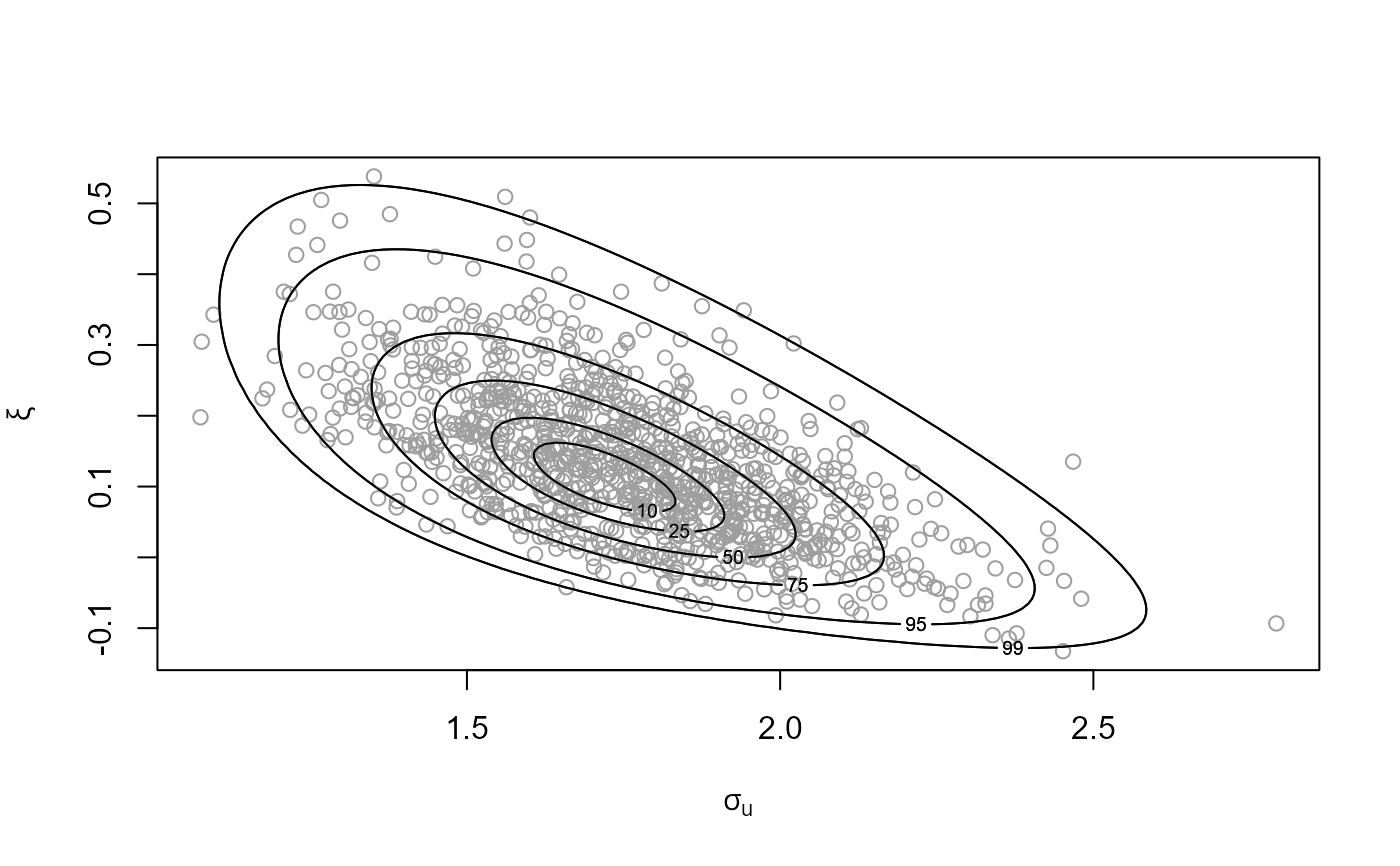
# GP model
u <- quantile(gom, probs = 0.65)
fp <- set_prior(prior = "flat", model = "gp", min_xi = -1)
gpg <- rpost_rcpp(n = 1000, model = "gp", prior = fp, thresh = u,
data = gom)
plot(gpg)
 # GP model, user-defined prior (same prior as the previous example)
ptr_gp_flat <- create_prior_xptr("gp_flat")
p_user <- set_prior(prior = ptr_gp_flat, model = "gp", min_xi = -1)
gpg <- rpost_rcpp(n = 1000, model = "gp", prior = p_user, thresh = u,
data = gom)
plot(gpg)
# GP model, user-defined prior (same prior as the previous example)
ptr_gp_flat <- create_prior_xptr("gp_flat")
p_user <- set_prior(prior = ptr_gp_flat, model = "gp", min_xi = -1)
gpg <- rpost_rcpp(n = 1000, model = "gp", prior = p_user, thresh = u,
data = gom)
plot(gpg)
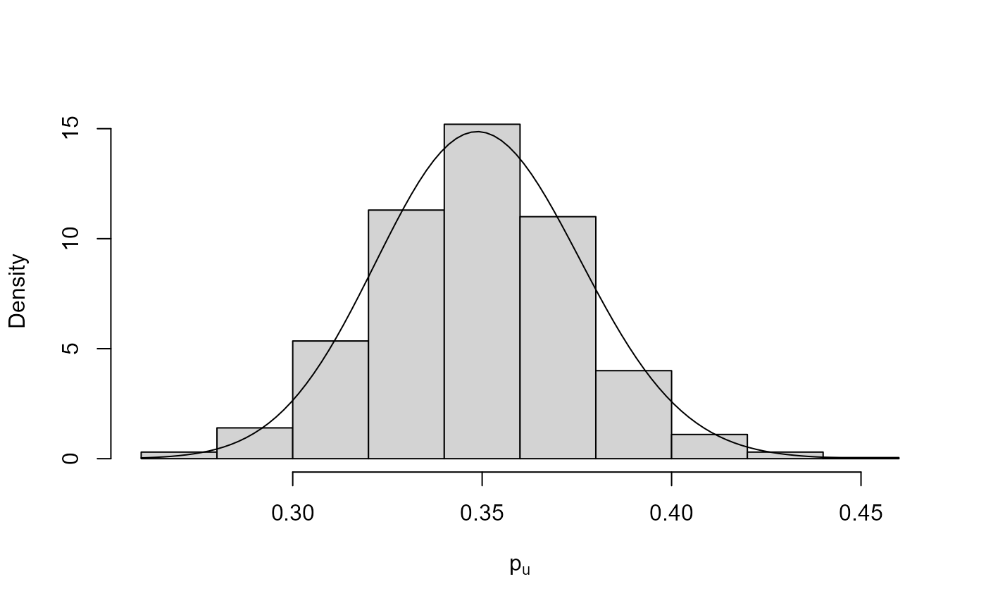
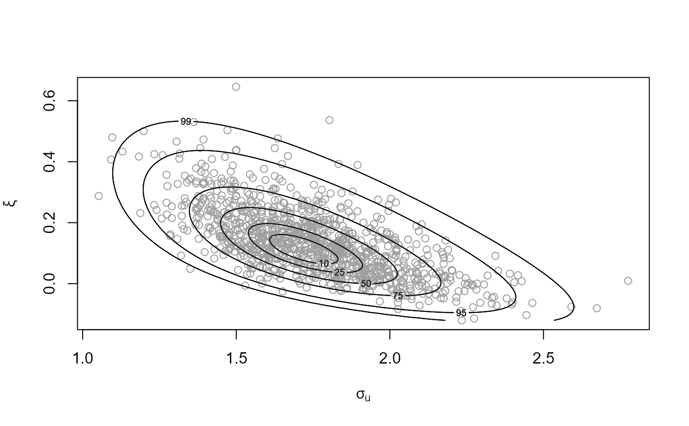 # Binomial-GP model
u <- quantile(gom, probs = 0.65)
fp <- set_prior(prior = "flat", model = "gp", min_xi = -1)
bp <- set_bin_prior(prior = "jeffreys")
bgpg <- rpost_rcpp(n = 1000, model = "bingp", prior = fp, thresh = u,
data = gom, bin_prior = bp)
plot(bgpg, pu_only = TRUE)
# Binomial-GP model
u <- quantile(gom, probs = 0.65)
fp <- set_prior(prior = "flat", model = "gp", min_xi = -1)
bp <- set_bin_prior(prior = "jeffreys")
bgpg <- rpost_rcpp(n = 1000, model = "bingp", prior = fp, thresh = u,
data = gom, bin_prior = bp)
plot(bgpg, pu_only = TRUE)
 plot(bgpg, add_pu = TRUE)
 # Setting the same binomial (Jeffreys) prior by hand
beta_prior_fn <- function(p, ab) {
return(stats::dbeta(p, shape1 = ab[1], shape2 = ab[2], log = TRUE))
}
jeffreys <- set_bin_prior(beta_prior_fn, ab = c(1 / 2, 1 / 2))
bgpg <- rpost_rcpp(n = 1000, model = "bingp", prior = fp, thresh = u,
data = gom, bin_prior = jeffreys)
plot(bgpg, pu_only = TRUE)
# Setting the same binomial (Jeffreys) prior by hand
beta_prior_fn <- function(p, ab) {
return(stats::dbeta(p, shape1 = ab[1], shape2 = ab[2], log = TRUE))
}
jeffreys <- set_bin_prior(beta_prior_fn, ab = c(1 / 2, 1 / 2))
bgpg <- rpost_rcpp(n = 1000, model = "bingp", prior = fp, thresh = u,
data = gom, bin_prior = jeffreys)
plot(bgpg, pu_only = TRUE)
 plot(bgpg, add_pu = TRUE)
 # GEV model
mat <- diag(c(10000, 10000, 100))
pn <- set_prior(prior = "norm", model = "gev", mean = c(0, 0, 0), cov = mat)
gevp <- rpost_rcpp(n = 1000, model = "gev", prior = pn, data = portpirie)
plot(gevp)
# GEV model
mat <- diag(c(10000, 10000, 100))
pn <- set_prior(prior = "norm", model = "gev", mean = c(0, 0, 0), cov = mat)
gevp <- rpost_rcpp(n = 1000, model = "gev", prior = pn, data = portpirie)
plot(gevp)
 # GEV model, user-defined prior (same prior as the previous example)
mat <- diag(c(10000, 10000, 100))
ptr_gev_norm <- create_prior_xptr("gev_norm")
pn_u <- set_prior(prior = ptr_gev_norm, model = "gev", mean = c(0, 0, 0),
icov = solve(mat))
gevu <- rpost_rcpp(n = 1000, model = "gev", prior = pn_u, data = portpirie)
plot(gevu)
# GEV model, user-defined prior (same prior as the previous example)
mat <- diag(c(10000, 10000, 100))
ptr_gev_norm <- create_prior_xptr("gev_norm")
pn_u <- set_prior(prior = ptr_gev_norm, model = "gev", mean = c(0, 0, 0),
icov = solve(mat))
gevu <- rpost_rcpp(n = 1000, model = "gev", prior = pn_u, data = portpirie)
plot(gevu)
 # GEV model, informative prior constructed on the probability scale
pip <- set_prior(quant = c(85, 88, 95), alpha = c(4, 2.5, 2.25, 0.25),
model = "gev", prior = "prob")
ox_post <- rpost_rcpp(n = 1000, model = "gev", prior = pip, data = oxford)
plot(ox_post)
# GEV model, informative prior constructed on the probability scale
pip <- set_prior(quant = c(85, 88, 95), alpha = c(4, 2.5, 2.25, 0.25),
model = "gev", prior = "prob")
ox_post <- rpost_rcpp(n = 1000, model = "gev", prior = pip, data = oxford)
plot(ox_post)
 # PP model
pf <- set_prior(prior = "flat", model = "gev", min_xi = -1)
ppr <- rpost_rcpp(n = 1000, model = "pp", prior = pf, data = rainfall,
thresh = 40, noy = 54)
plot(ppr)
# PP model
pf <- set_prior(prior = "flat", model = "gev", min_xi = -1)
ppr <- rpost_rcpp(n = 1000, model = "pp", prior = pf, data = rainfall,
thresh = 40, noy = 54)
plot(ppr)
 # PP model, user-defined prior (same prior as the previous example)
ptr_gev_flat <- create_prior_xptr("gev_flat")
pf_u <- set_prior(prior = ptr_gev_flat, model = "gev", min_xi = -1,
max_xi = Inf)
ppru <- rpost_rcpp(n = 1000, model = "pp", prior = pf_u, data = rainfall,
thresh = 40, noy = 54)
plot(ppru)
# PP model, user-defined prior (same prior as the previous example)
ptr_gev_flat <- create_prior_xptr("gev_flat")
pf_u <- set_prior(prior = ptr_gev_flat, model = "gev", min_xi = -1,
max_xi = Inf)
ppru <- rpost_rcpp(n = 1000, model = "pp", prior = pf_u, data = rainfall,
thresh = 40, noy = 54)
plot(ppru)
 # PP model, informative prior constructed on the quantile scale
piq <- set_prior(prob = 10^-(1:3), shape = c(38.9, 7.1, 47),
scale = c(1.5, 6.3, 2.6), model = "gev", prior = "quant")
rn_post <- rpost_rcpp(n = 1000, model = "pp", prior = piq, data = rainfall,
thresh = 40, noy = 54)
plot(rn_post)
# PP model, informative prior constructed on the quantile scale
piq <- set_prior(prob = 10^-(1:3), shape = c(38.9, 7.1, 47),
scale = c(1.5, 6.3, 2.6), model = "gev", prior = "quant")
rn_post <- rpost_rcpp(n = 1000, model = "pp", prior = piq, data = rainfall,
thresh = 40, noy = 54)
plot(rn_post)
 # OS model
mat <- diag(c(10000, 10000, 100))
pv <- set_prior(prior = "norm", model = "gev", mean = c(0, 0, 0), cov = mat)
osv <- rpost_rcpp(n = 1000, model = "os", prior = pv, data = venice)
plot(osv)
# OS model
mat <- diag(c(10000, 10000, 100))
pv <- set_prior(prior = "norm", model = "gev", mean = c(0, 0, 0), cov = mat)
osv <- rpost_rcpp(n = 1000, model = "os", prior = pv, data = venice)
plot(osv)
