EVA 2021 revdbayes exercises 2
EV inference using revdbayes
Source:vignettes/ex2revdbayes.Rmd
ex2revdbayes.RmdGetting started
- Install RStudio Desktop (if you do not already have it) and open it
- Save ex2revdbayes.Rmd to your computer (there is also a link to it above)
- Open
ex2revdbayes.Rmdin Rstudio - The R code is arranged in chunks highlighted in grey
- You can run the code in a chunk by clicking on the green triangle on the top right of the chunk
- There is information about Exercises 2 (and Exercises 1) in the EVA2021 revdbayes slides
Aims
- Compare ROU approaches for sampling from a GP posterior
- Perform posterior predictive checking and inference
- Consider how to sample efficiently from a PP posterior
- Compare
revdbayesandevdbayesfor sampling from a GEV posterior
There is further information in the Introduction to revdbayes vignette.
# We need the evdbayes, revdbayes, ggplot2, bayesplot and coda packages
pkg <- c("evdbayes", "revdbayes", "ggplot2", "bayesplot", "coda")
pkg_list <- pkg[!pkg %in% installed.packages()[, "Package"]]
install.packages(pkg_list)
## package 'evdbayes' successfully unpacked and MD5 sums checked
## package 'coda' successfully unpacked and MD5 sums checked
##
## The downloaded binary packages are in
## C:\Users\Paul\AppData\Local\Temp\RtmpAJHHah\downloaded_packages## Warning: package 'coda' was built under R version 4.5.3
# Simulation sample size
n <- 10000
GP model for threshold excesses
GP posteriors
# Information about the rpost function
?rpost
# Information about the gom (significant wave heights) data
?gom
# Sample on (sigma_u, xi) scale
gp1 <- rpost(n = n, model = "gp", prior = fp, thresh = u, data = gom,
rotate = FALSE)
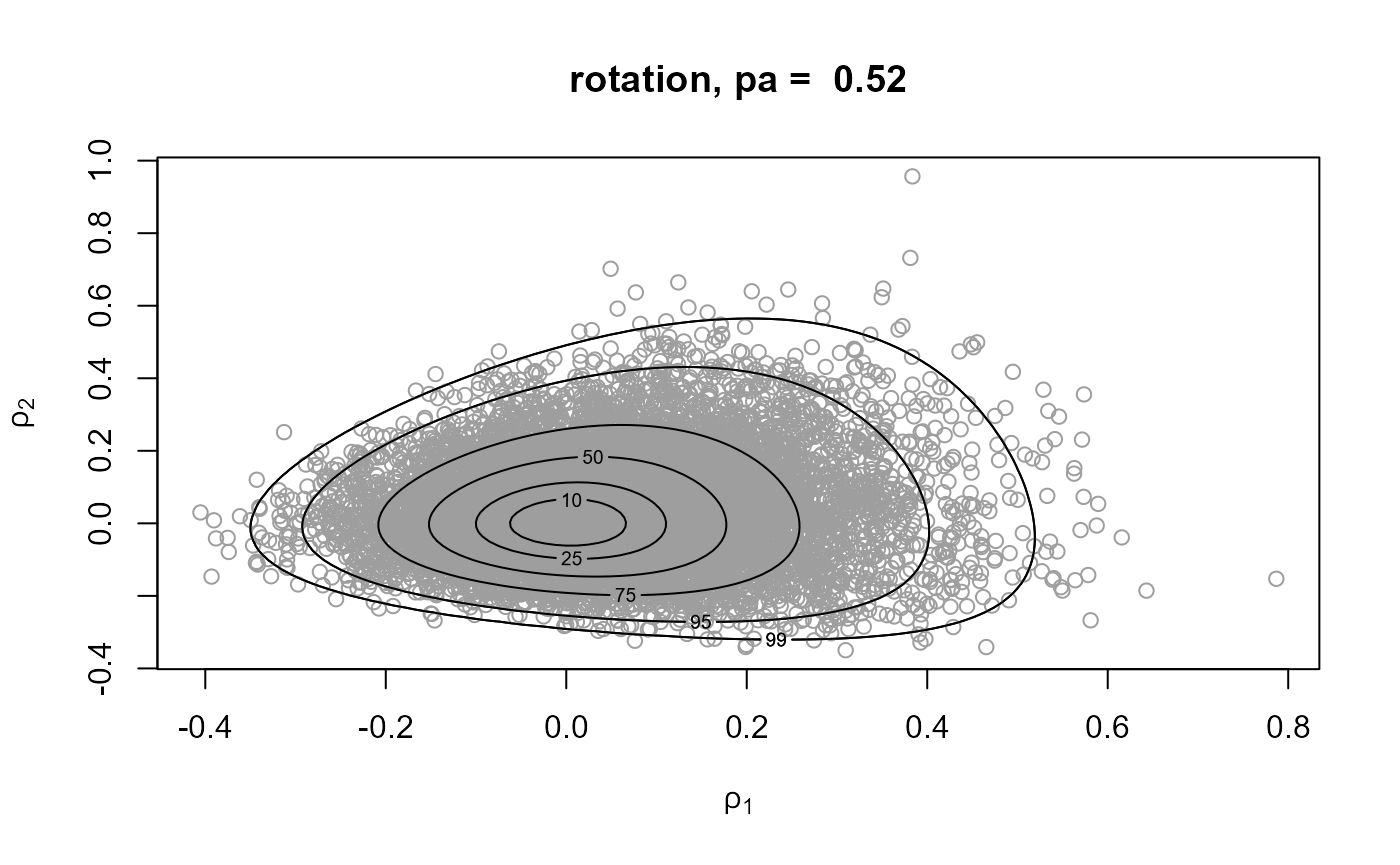
# Rotation
gp2 <- rpost(n = n, model = "gp", prior = fp, thresh = u, data = gom)
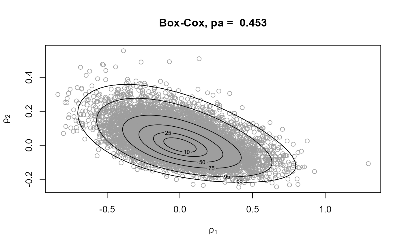
# Box-Cox transformation (after transformation to positivity)
gp3 <- rpost(n = n, model = "gp", prior = fp, thresh = u, data = gom,
rotate = FALSE, trans = "BC")
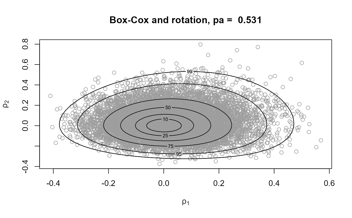
# Box-Cox transformation and then rotation
gp4 <- rpost(n = n, model = "gp", prior = fp, thresh = u, data = gom,
trans = "BC")Comparing approaches
# Samples and posterior density contours
plot(gp1, main = paste("mode relocation only, pa = ", round(gp1$pa, 3)))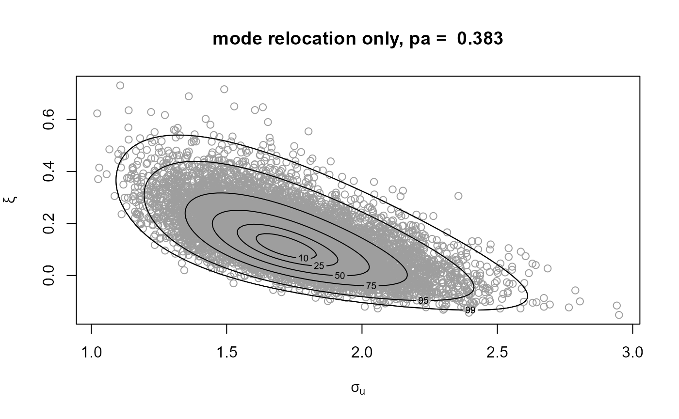
rpost_rcpp() is faster than rpost(). See
the rusting
faster vignette.
gp2 <- rpost_rcpp(n = n, model = "gp", prior = fp, thresh = u, data = gom)Suggestion: increase the threshold and see how the appearance of the posterior changes.
Posterior predictive checking
There is further information in the Posterior predictive EV inference vignette.
# nrep = 50 asks for 50 fake replicates of the original data
# For each of 50 posterior samples of the parameters a dataset is simulated
gpg <- rpost(n = n, model = "gp", prior = fp, thresh = u, data = gom,
             nrep = 50)
# Information about pp_check.evpost
?pp_check.evpost
# Compare real and fake datasets
pp_check(gpg, type = "multiple", subtype = "dens") + ggtitle("GP kernel density estimates")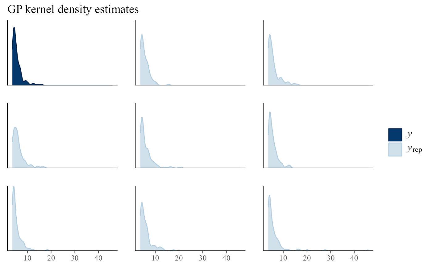
# Compare real and fake summary statistics
pp_check(gpg, stat = "max")
## `stat_bin()` using `bins = 30`. Pick better value `binwidth`.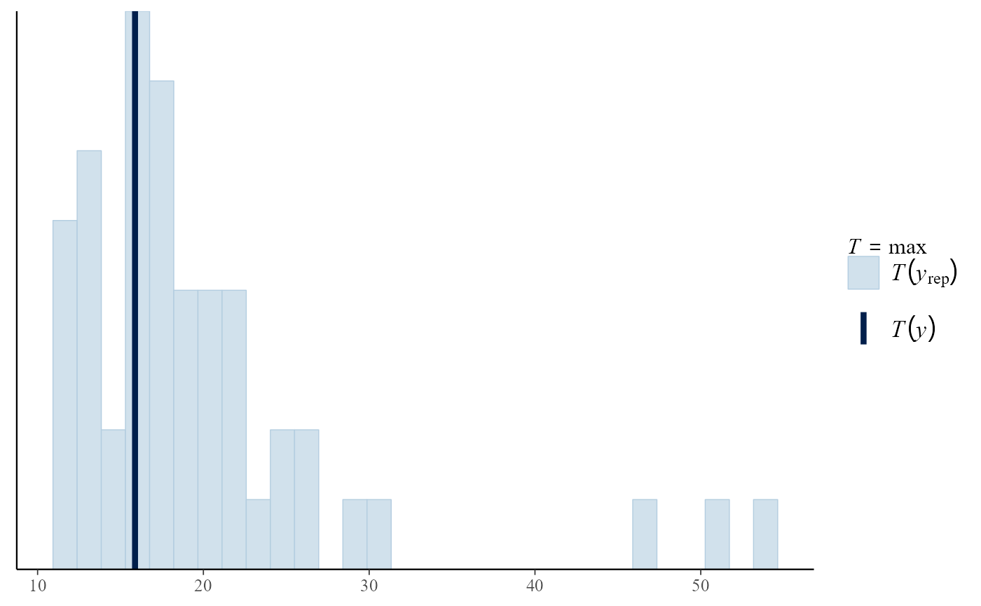
- Would you be able to spot the real dataset or summary statistic if it was not highlighted?
- Option: you could play with the arguments
-
typeand/orsubtypefor the first plot -
statfor the second plot
-
Posterior predictive EV inference
Binomial-GP model for threshold exceedances
Modelling threshold excesses is only part of the story. We also need to model the proportion of observations that exceed the threshold.
bp <- set_bin_prior(prior = "jeffreys")
# We need to provide the mean number of observations per year
# The data cover a period of 105 years
npy_gom <- length(gom)/105
bgpg <- rpost(n = 1000, model = "bingp", prior = fp, thresh = u, data = gom,
              bin_prior = bp, npy = npy_gom, nrep = 50)
We can make predictive inferences about the largest value \(M_N\) to be observed over a time horizon of \(N\) years.
# Information about pp_check.evpost
?predict.evpost
# Predictive density of the largest value in `n_years' years
plot(predict(bgpg, type = "d", n_years = 200))
# Predictive intervals (equi-tailed and shortest possible)
i_bgpp <- predict(bgpg, n_years = 200, level = c(95, 99), hpd = TRUE)
plot(i_bgpp, which_int = "both")
## Warning in graphics::par(u): argument 1 does not name a graphical parameter
i_bgpp$short ## lower upper n_years level
## [1,] 10.315968 39.90904 200 95
## [2,] 9.396545 73.17092 200 99
# The predictive 100, 200 and 500 year return levels
predict(bgpg, type = "q", n_years = 1, x = c(0.99, 0.995, 0.998))$y
## [,1]
## [1,] 15.22621
## [2,] 18.09992
## [3,] 22.97870See Northrop and Attalides (2017) for an analysis of these data using an informative prior.
PP model for threshold exceedances
We compare three ways to sample from a PP posterior distribution
- Parameterise in terms of annual maxima
- Wadsworth et al. (2010): parameterise to make \(\mu\) orthogonal to \((\sigma, \xi)\)
- Empirical rotation to reduce association
# Information about the rainfall data
?revdbayes::rainfall
# Set a threshold and use the prior from the evdbayes user guide
rthresh <- 40
prrain <- evdbayes::prior.quant(shape = c(38.9,7.1,47), scale = c(1.5,6.3,2.6))
# 1. Number of blocks = number of years of data (54)
r1 <- rpost(n = n, model = "pp", prior = prrain, data = rainfall,
            thresh = rthresh, noy = 54, rotate = FALSE)
plot(r1)
# 2. Number of blocks = number of threshold excesses (use_noy = FALSE)
n_exc <- sum(rainfall > rthresh, na.rm = TRUE)
r2 <- rpost(n = n, model = "pp", prior = prrain, data = rainfall,
            thresh = rthresh, noy = 54, use_noy = FALSE, rotate = FALSE)
plot(r2, ru_scale = TRUE)
# 3. # Rotation about maximum a posteriori estimate (MAP)
r3 <- rpost(n = n, model = "pp", prior = prrain, data = rainfall,
            thresh = rthresh, noy = 54)
plot(r3, ru_scale = TRUE)
c(r1$pa, r2$pa, r3$pa)## [1] 0.1717003 0.1936333 0.2988375- Based on the plots, which approach do you expect to have the largest probability of acceptance?
- Is this what you see in the values of
r1$pa,r2$paandr3$pa?
GEV model for block maxima
# Information about the portpirie data
?revdbayes::portpirie
# Use the prior from the evdbayes user guide
mat <- diag(c(10000, 10000, 100))
pn <- set_prior(prior = "norm", model = "gev", mean = c(0, 0, 0), cov = mat)
revdbayes
mat <- diag(c(10000, 10000, 100))
gevp  <- rpost_rcpp(n = n, model = "gev", prior = pn, data = portpirie)
# Information about plot.evpost
?plot.evpost
# Can use the plots from the bayesplot package
plot(gevp, use_bayesplot = TRUE, fun_name = "dens")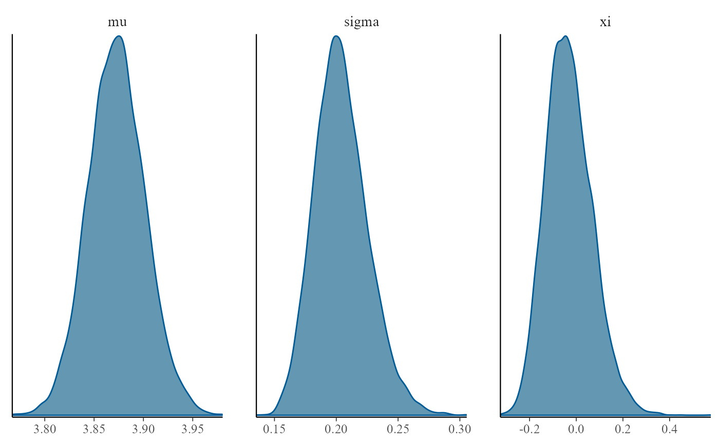
plot(gevp, use_bayesplot = TRUE, pars = "xi", prob = 0.95)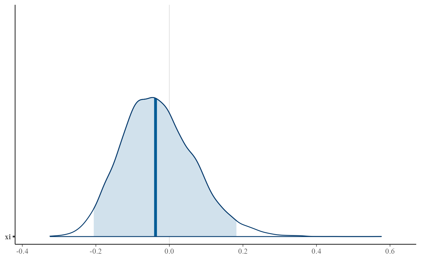
evdbayes
# evdbayes has a function ar.choice to help set the proposal SDs
# It does this by searching for values that achieve approximately
# target values for the acceptance rates (default 0.4 for all parameters)
?ar.choice
# Initialise evdbayes' Markov chain at the estimated posterior mean
init <- colMeans(gevp$sim_vals)
prop.sd.auto <- ar.choice(init = init, prior = pn, lh = "gev",
                          data = portpirie, psd = rep(0.01, 3),
                          tol = rep(0.02, 3))$psd
post <- posterior(n, init = init, prior = pn, lh = "gev",
                  data = portpirie, psd = prop.sd.auto)
for (i in 1:3) plot(post[, i], ylab = c("mu","sigma","xi")[i]) 


post_for_coda <- coda::mcmc(post)
# Assuming no burn-in period
burnin <- 0
post_for_coda <- window(post_for_coda, start = burnin + 1)
# Trace plots and KDEs
plot(post_for_coda)
# The sampled values are autocorrelated
coda::acfplot(post_for_coda)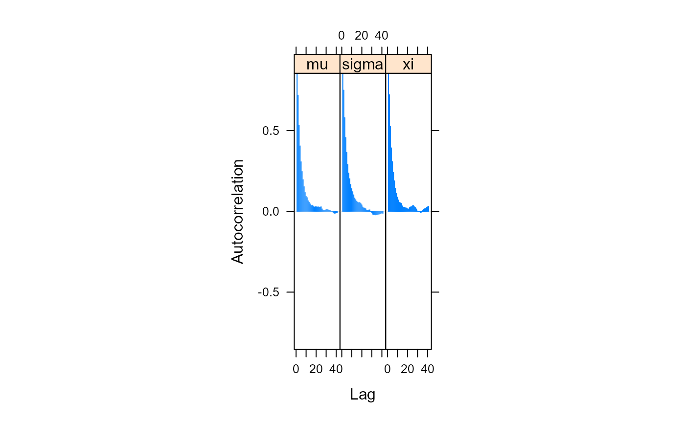
# Effective sample sizes (10,000 for revdbayes)
coda::effectiveSize(post_for_coda)
## mu sigma xi
## 1530.996 1418.982 1589.088- In practice one would run multiple chains and use the Gelman-Rubin
convergence diagnostic, e.g.
gelman.diagin thecodapackage. - The Introduction
to revdbayes shows that the posterior samples from
evdbayesandrevdbayesare in agreement.