Posterior predictive checks for an evpost object — pp

pp_check method for class "evpost". This provides an interface to the functions that perform posterior predictive checks in the bayesplot package. See PPC-overview for details of these functions.

Usage

# S3 method for class 'evpost'
pp_check(
  object,
  ...,
  type = c("stat", "overlaid", "multiple", "intervals", "user"),
  subtype = NULL,
  stat = "median",
  nrep = 8,
  fun = NULL
)

Arguments

object

An object of class "evpost", a result of a call to rpost or rpost_rcpp. Currently object$model = "gev", "gp", "bingp" and "pp" are supported.

...

Additional arguments passed on to bayesplot functions.

type

A character vector. The type of bayesplot plot required:

"stat" for predictive test statistics (see PPC-test-statistics),
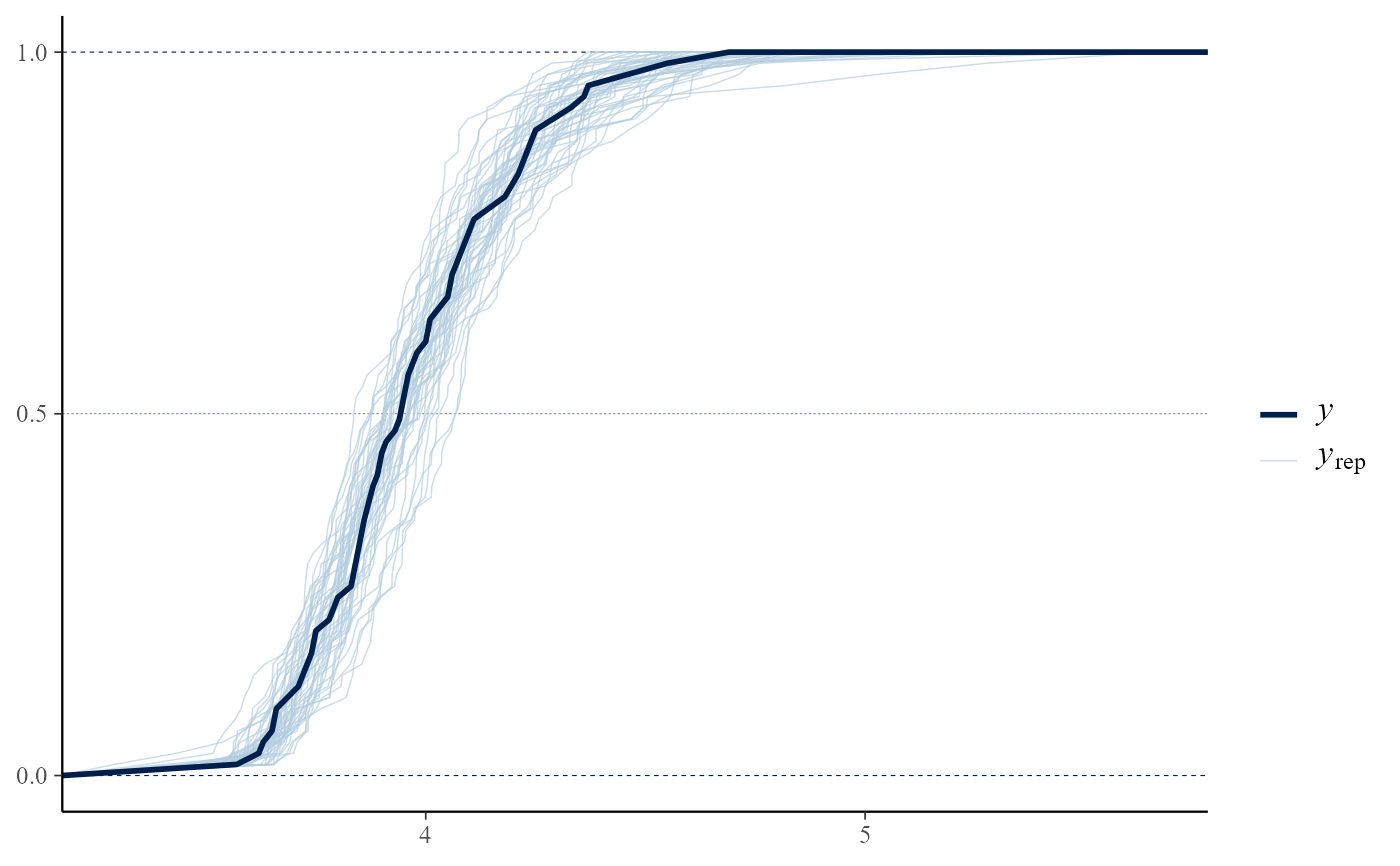
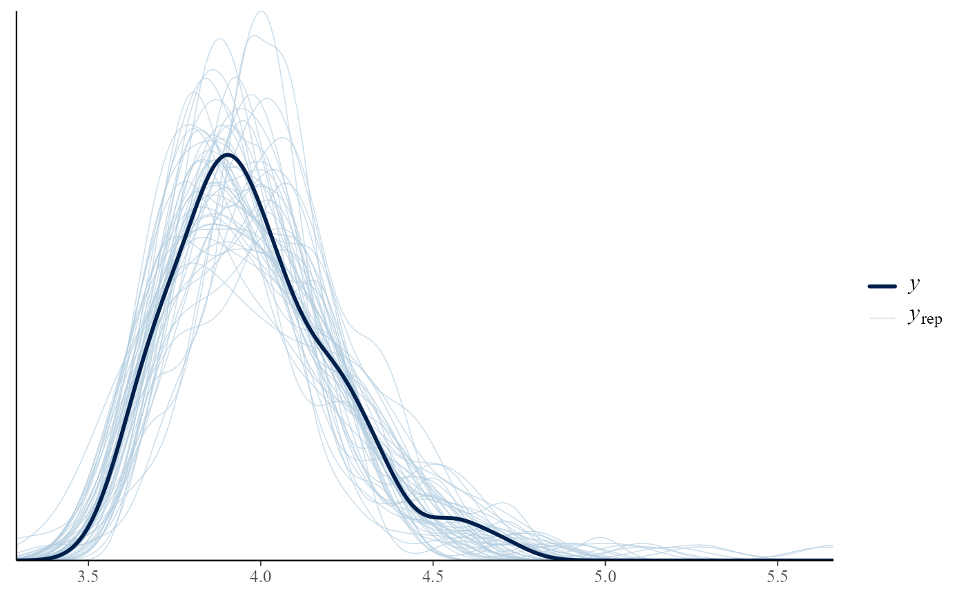
"overlaid" for comparison of observed data to predictive simulated datasets using overlaid density function or distribution functions (see PPC-distributions),
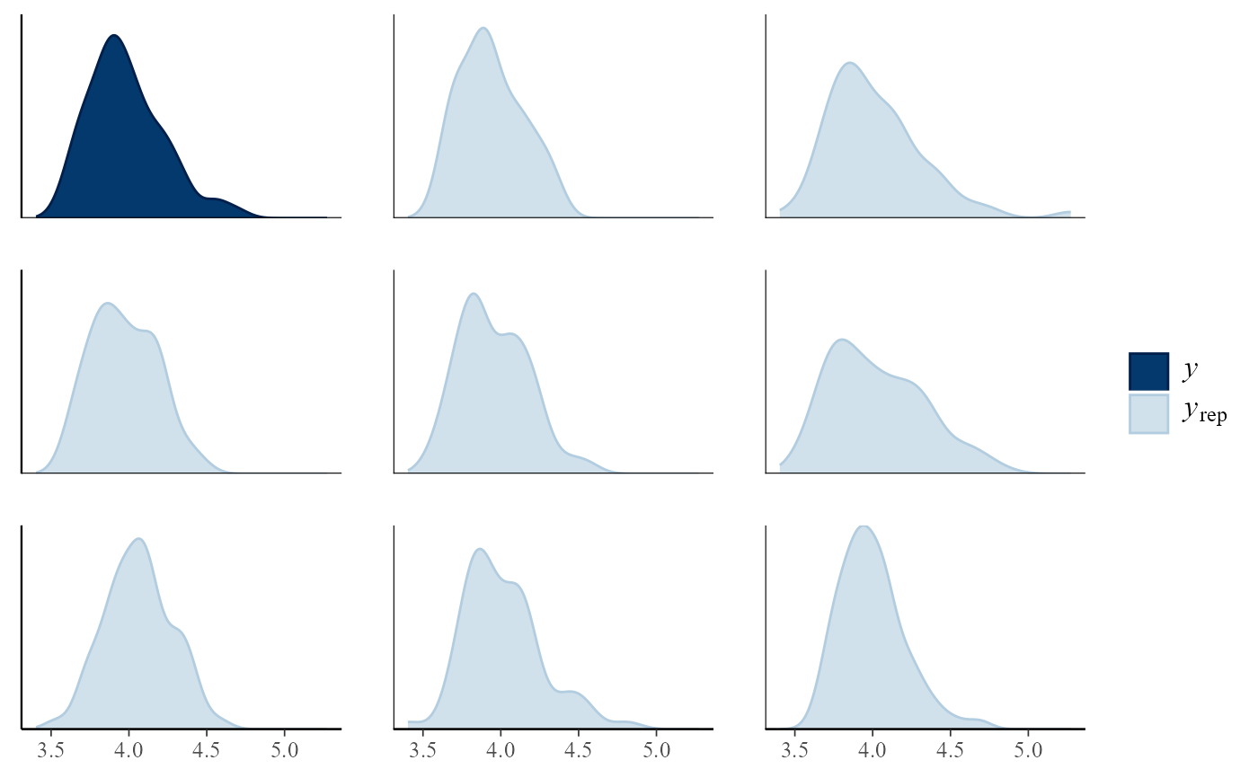
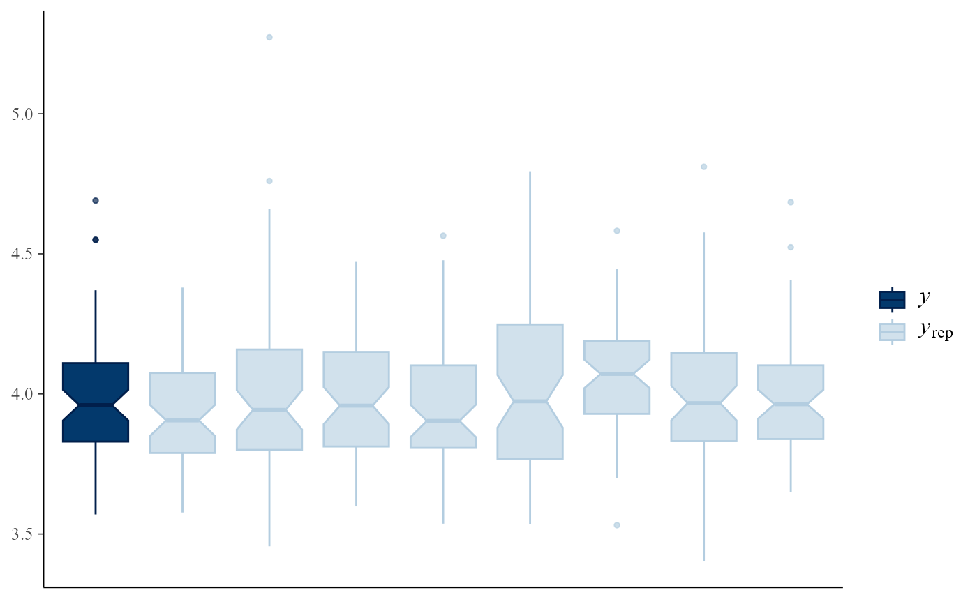
"multiple" for comparison of observed data to predictive simulated datasets using multiple summary plots (see PPC-distributions),
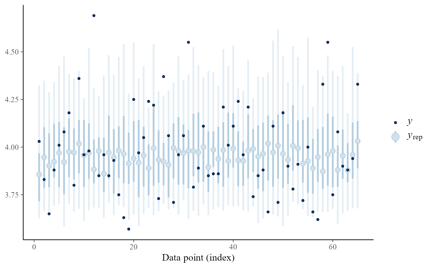
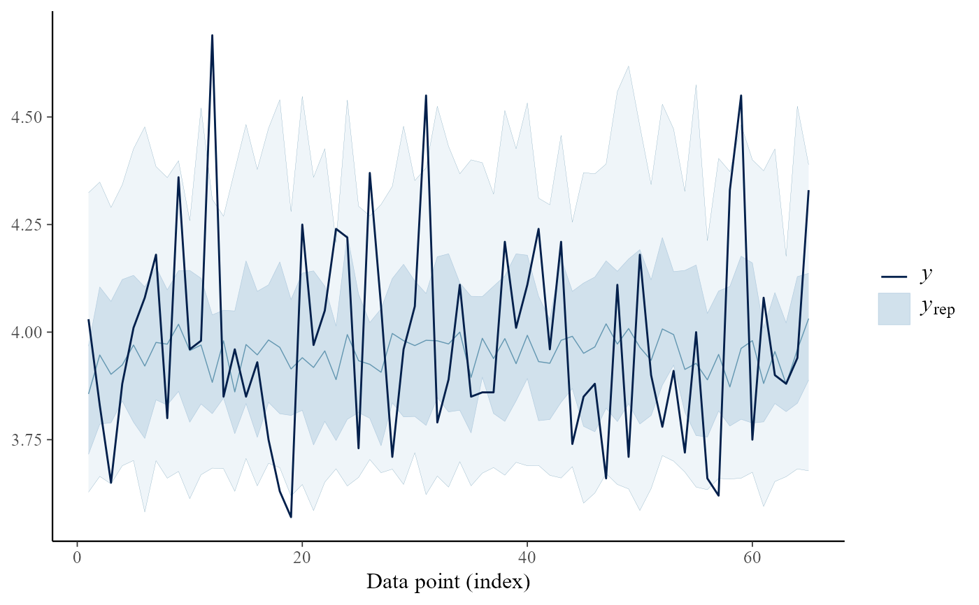
"intervals" for comparison of observed data to predictive simulated datasets using sample medians and a predictive interval, (see PPC-intervals),
"user" for direct access to the default bayesplot function pp_check. This requires the argument fun to be supplied (see pp_check).

subtype

A character scalar. Specifies the form of the plot(s) produced. Could be one of "dens", "hist", "boxplot", "ribbon" or "intervals". If subtype is not supplied then the defaults are: "ecdf" if type = overlaid, "dens" if type = multiple, "intervals" if type = intervals. subtype is not relevant if type = "stat".

stat

See PPC-test-statistics.

nrep

If type = "multiple" the maximum number of summary plots of the predictive simulated datasets to include. If nrep is greater than nrow(object$data_rep) then nrep is set equal to nrow(object$data_rep).

fun

The plotting function to call. Only relevant if type = "user". Can be any of the functions detailed at PPC-overview. The "ppc_" prefix can optionally be dropped if fun is specified as a string.

Value

A ggplot object that can be further customized using the ggplot2 package.

Details

For details of these functions see PPC-overview. See also the vignette Posterior Predictive Extreme Value Inference and the bayesplot vignette Graphical posterior predictive checks.

The general idea is to compare the observed data object$data with a matrix object$data_rep in which each row is a replication of the observed data simulated from the posterior predictive distribution. For greater detail see Chapter 6 of Gelman et al. (2013).

The format of object$data depends on the model:

model = "gev". A vector of block maxima.
model = "gp". Data that lie above the threshold, i.e. threshold exceedances.
model = "bingp" or model = "pp". The input data are returned but any value lying below the threshold is set to object$thresh.

In all cases any missing values have been removed from the data.

If model = "bingp" or "pp" the rate of threshold exceedance is part of the inference. Therefore, the number of values in object$data_rep that lie above the threshold varies between predictive replications, with values below the threshold being left-censored at the threshold. This limits a little the posterior predictive checks that it is useful to perform. In the examples below we have compared object$data and object$data_rep using only their sample maxima.

References

Jonah Gabry (2016). bayesplot: Plotting for Bayesian Models. R package version 1.1.0. https://CRAN.R-project.org/package=bayesplot

Gelman, A., Carlin, J. B., Stern, H. S., Dunson, D. B., Vehtari, A., and Rubin, D. B. (2013). Bayesian Data Analysis. Chapman & Hall/CRC Press, London, third edition. (Chapter 6)

Examples

# \donttest{
# GEV model
data(portpirie)
mat <- diag(c(10000, 10000, 100))
pn <- set_prior(prior = "norm", model = "gev", mean = c(0,0,0), cov = mat)
gevp  <- rpost(1000, model = "gev", prior = pn, data = portpirie,
               nrep = 50)

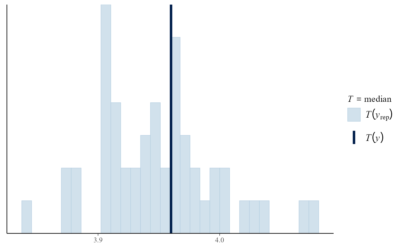
# Posterior predictive test statistics
pp_check(gevp)
#> `stat_bin()` using `bins = 30`. Pick better value `binwidth`.

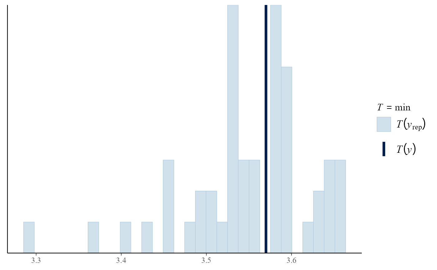
pp_check(gevp, stat = "min")
#> `stat_bin()` using `bins = 30`. Pick better value `binwidth`.

pp_check(gevp, stat = c("min", "max"))

iqr <- function(y) diff(quantile(y, c(0.25, 0.75)))
pp_check(gevp, stat = "iqr")
#> Error in get(as.character(FUN), mode = "function", envir = envir): object 'iqr' of mode 'function' was not found

# Overlaid density and distributions functions
pp_check(gevp, type = "overlaid")

pp_check(gevp, type = "overlaid", subtype = "dens")


# Multiple plots
pp_check(gevp, type = "multiple")

pp_check(gevp, type = "multiple", subtype = "hist")
#> `stat_bin()` using `bins = 30`. Pick better value `binwidth`.

pp_check(gevp, type = "multiple", subtype = "boxplot")


# Intervals
pp_check(gevp, type = "intervals")
#> Warning: Using `size` aesthetic for lines was deprecated in ggplot2 3.4.0.
#> ℹ Please use `linewidth` instead.
#> ℹ The deprecated feature was likely used in the bayesplot package.
#>   Please report the issue at <https://github.com/stan-dev/bayesplot/issues/>.

pp_check(gevp, type = "intervals", subtype = "ribbon")


# User-supplied bayesplot function
# Equivalent to p_check(gevp, type = "overlaid")
pp_check(gevp, type = "user", fun = "dens_overlay")


# GP model
u <- quantile(gom, probs = 0.65)
fp <- set_prior(prior = "flat", model = "gp", min_xi = -1)
gpg <- rpost(n = 1000, model = "gp", prior = fp, thresh = u,
             data = gom, nrep = 50)
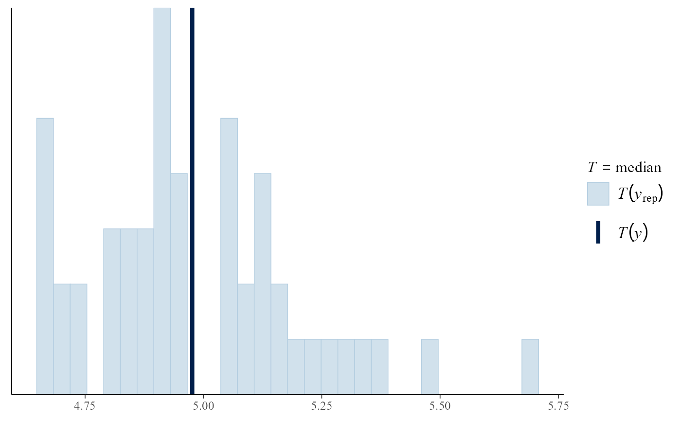
pp_check(gpg)
#> `stat_bin()` using `bins = 30`. Pick better value `binwidth`.

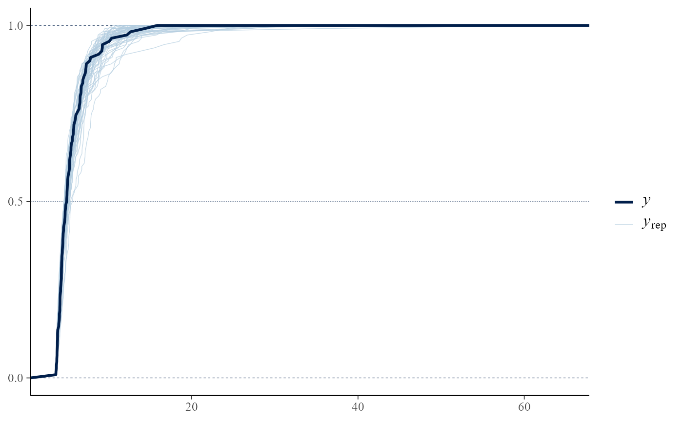
pp_check(gpg, type = "overlaid")


# bin-GP model
bp <- set_bin_prior(prior = "jeffreys")
bgpg <- rpost(n = 1000, model = "bingp", prior = fp, thresh = u,
              data = gom, bin_prior = bp, nrep = 50)
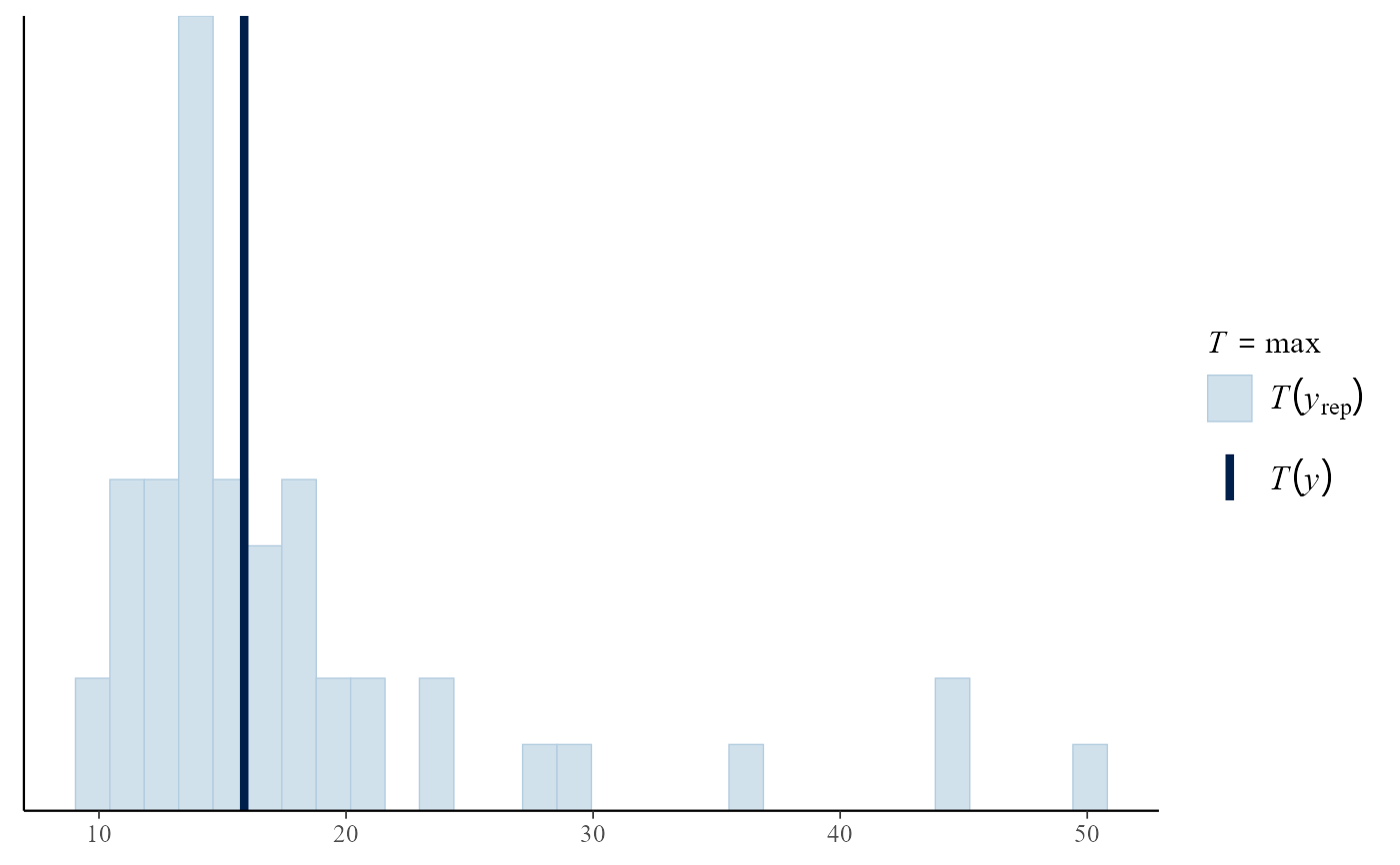
pp_check(bgpg, stat = "max")
#> `stat_bin()` using `bins = 30`. Pick better value `binwidth`.


# PP model
data(rainfall)
rthresh <- 40
pf <- set_prior(prior = "flat", model = "gev", min_xi = -1)
ppr <- rpost(n = 1000, model = "pp", prior = pf, data = rainfall,
             thresh = rthresh, noy = 54, nrep = 50)
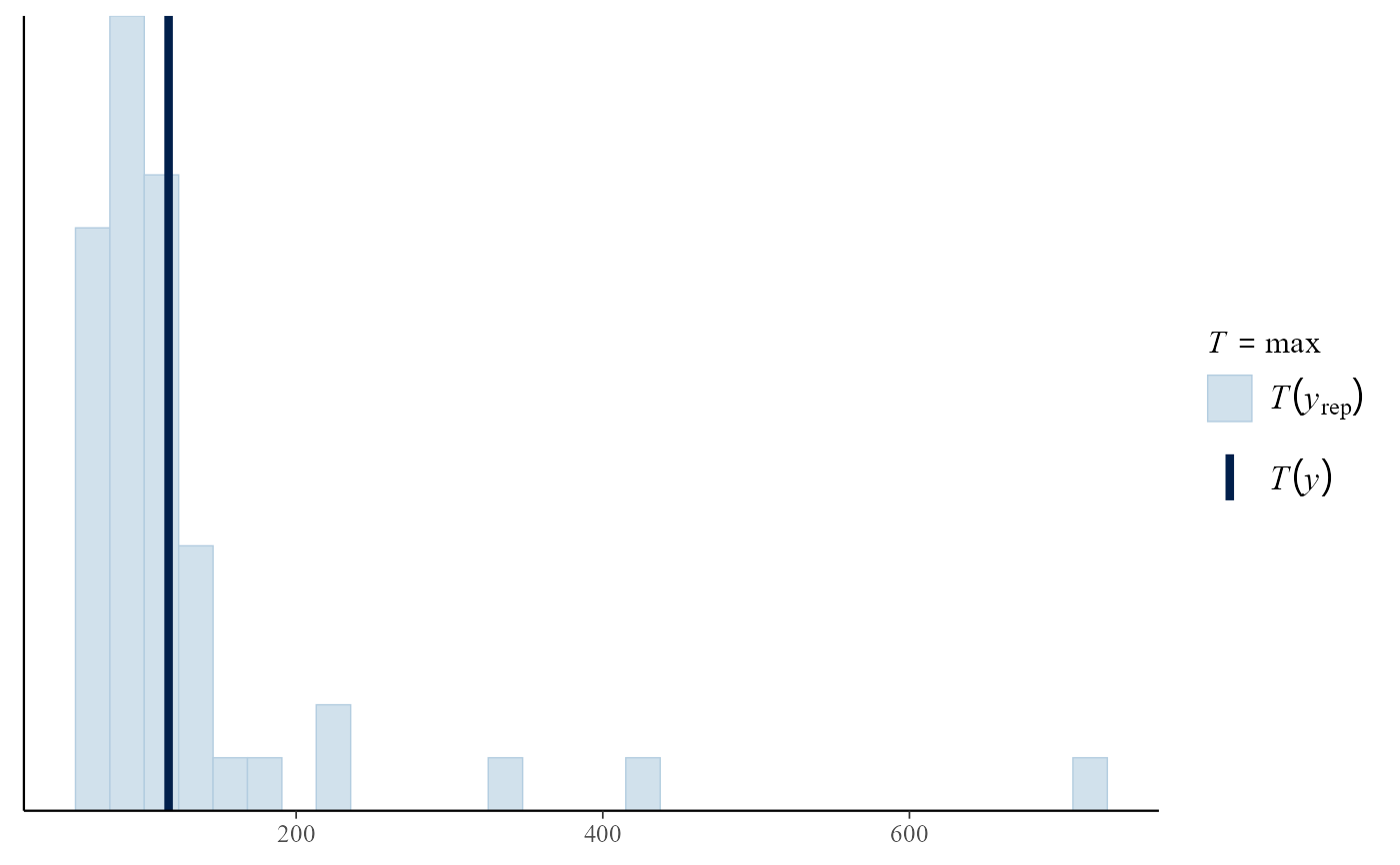
pp_check(ppr, stat = "max")
#> `stat_bin()` using `bins = 30`. Pick better value `binwidth`.

# }