Introducing threshr: Threshold Selection and Uncertainty for Extreme Value Analysis
Paul J. Northrop
2026-03-24
Source:vignettes/threshr-vignette.Rmd
threshr-vignette.RmdThe threshr package deals primarily with the selection of thresholds for use in extreme value modelling. The underlying methodology is described in detail in Northrop, Attalides, and Jonathan (2017). Bayesian leave-one-out cross-validation is used to compare the extreme value predictive performance resulting from each of a set of thresholds. This assesses the trade-off between the model mis-specification bias that results from an inappropriately low threshold and the loss of precision of estimation from an unnecessarily high threshold. There many other approaches to address this bias-variance trade-off. See Scarrott and MacDonald (2012) for a review.
At the moment only the simplest case, where the data can be treated as independent identically distributed observations, is considered. In this case the model used is a combination of a binomial distribution for the number of exceedances of a given threshold and a generalized Pareto (GP) distribution for the amounts, the threshold excesses by which exceedances lie above a threshold. We refer to this as a binomial-GP model. Future releases of threshr will tackle more general situations.
We use the function ithresh to compare the predictive
performances of each of a set of user-supplied thresholds. We also
perform predictive inferences for future extreme values, using the
predict method for objects returned from
ithresh. These inferences can be based either on a single
threshold or on a weighted average of inferences from multiple
thresholds. The weighting reflects an estimated measure of the
predictive performance of the threshold and can also incorporate
user-supplied prior probabilities for each threshold.
A traditional simple graphical method to inform threshold selection
is to plot estimates of, and confidence intervals for, the GP shape
parameter \(\xi\) over a range of
thresholds. This plot is used to choose a threshold above which the
underlying GP shape parameter may be approximately constant. See Chapter
4 of Coles (2001) for details. Identifying
a single threshold using this method is usually unrealistic but the plot
can point to a range of thresholds that merit more sophisticated
analysis. The threshr function stability
produces this type of plot.
Cross-validatory predictive performance for i.i.d. data
We provide a brief outline of the methodology underlying
ithresh. For full details see Northrop, Attalides, and Jonathan (2017).
Consider a set of training thresholds \(u_1, \ldots, u_k\). The validation
threshold \(v = u_k\) defines
validation data: indicators of whether or not an observation exceeds
\(v\) and, if it does, the amount by
which \(v\) is exceeded. For a given
training threshold leave-one-out cross-validation estimates the quality
of predictive inference for each of the individual omitted samples based
on Bayesian inferences from a binomial-GP model. Importance sampling is
used to reduce computation time: only two posterior samples are required
for each training threshold. Simulation from the posterior distributions
of the binomial-GP parameters is performed using the
revdbayes package (Northrop
2017).
In the first release of threshr the binomial
probability is assumed to be independent of the parameters of the GP
distribution a priori. This will be relaxed in a later release.
The user can choose from a selection of in-built prior distributions and
may specify their own prior for GP models parameters. By default the
Beta(1/2, 1/2) Jeffreys’ prior is used for the threshold exceedance
probability of the binomial distribution and a generalization of the
Maximal Data Information (MDI) prior is used for the GP parameters. See
the documentation of ithresh and Northrop, Attalides, and Jonathan (2017) for
details of the latter.
We use the storm peak significant wave heights datasets analysed in
Northrop, Attalides, and Jonathan (2017)
from the Gulf of Mexico (gom, with 315 observations) and
the northern North Sea (ns, with 628 observations) to
illustrate the code. There should be enough exceedances of the
validation threshold \(v = u_k\) to
enable the predictive performances of the training thresholds to be
compared. Jonathan and Ewans (2013)
recommend that when making inferences about a GP distribution there
should be no fewer than 50 exceedances. We bear this rule-of-thumb in
mind when setting the vectors of training thresholds below.
library(threshr)

# Set the size of the posterior sample simulated at each threshold
n <- 10000

## North Sea significant wave heights

# Set a vector of training thresholds
u_vec_ns <- quantile(ns, probs = seq(0.1, 0.85, by = 0.05))
# Compare the predictive performances of the training thresholds
ns_cv <- ithresh(data = ns, u_vec = u_vec_ns, n = n)

## Gulf of Mexico significant wave heights

# Set a vector of training thresholds
u_vec_gom <- quantile(gom, probs = seq(0.1, 0.8, by = 0.05))
# Compare the predictive performances of the training thresholds
gom_cv <- ithresh(data = gom, u_vec = u_vec_gom, n = n)
The default plot method for objects returned by ithresh
is of the estimated measures of predictive performance, normalized to
sum to 1, against training threshold. See equations (7) and (14) of
Northrop, Attalides, and Jonathan
(2017).
plot(ns_cv, lwd = 2, cex.axis = 0.8)
mtext("North Sea : significant wave height / m", side = 3, line = 2.5)

plot(gom_cv, lwd = 2, cex.axis = 0.8)
mtext("Gulf of Mexico: significant wave height / m", side = 3, line = 2.5)

The summary method identifies which training threshold is estimated to perform best.
summary(ns_cv)
#> v v quantile best u best u quantile index of u_vec
#> 1 5.6972 85 2.204 25 4
summary(gom_cv)
#> v v quantile best u best u quantile index of u_vec
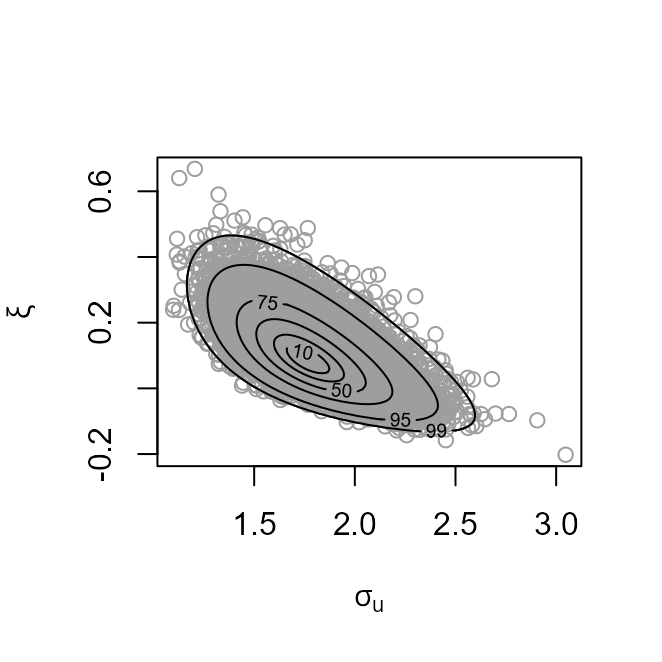
#> 1 4.607 80 3.3878 60 11The plot method can also produce a plot of the posterior sample of
the GP parameters generated using a training threshold chosen by the
user, e.g. the argument which_u = 5 specifies the fifth
element of the vector of training thresholds, or using the best
threshold, as below.
# Plot of Generalized Pareto posterior sample at the best threshold
# (based on the lowest validation threshold)
plot(ns_cv, which_u = "best")
plot(gom_cv, which_u = "best")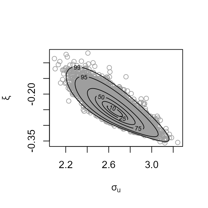
Predictive inference for future extremes
Let \(M_N\) denote the largest value
to be observed in a time period of length \(N\) years. The predict method for objects
returned from ithresh performs predictive inference for
\(M_N\) based either on a single
training threshold or on a weighted average of inferences from multiple
training thresholds.
Single training threshold
By default the threshold that is estimated to perform best is used. A
different threshold can be selected using the argument
which_u. Using type = "d" produces the
predictive density function. The values of \(N\) can be set using n_years.
The default is \(N = 100\).
# Predictive distribution function
best_p <- predict(gom_cv, n_years = c(100, 1000), type = "d")
plot(best_p)
Inferences averaged over multiple thresholds
This option is selected using which_u = "all". The user
can specify a prior probability for each threshold using
u_prior. The default is that all thresholds receive equal
prior probability, in which case the weights applied to individual
training thresholds are those displayed in the threshold diagnostic plot
above. The default, type = "p" produces the predictive
distribution function. If which_u = "all" then
n_years must have length one. The default is \(N = 100\).
### All thresholds plus weighted average of inferences over all thresholds
all_p <- predict(gom_cv, which_u = "all")
plot(all_p)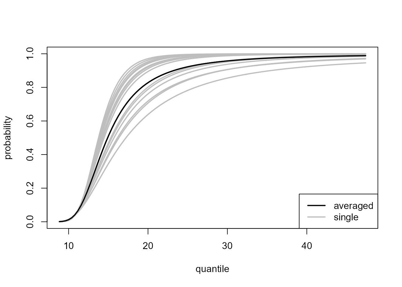
As we expect, the estimated distribution function obtained by the weighted average over all thresholds lies between the pointwise envelope of the curves of the individual thresholds.