Chapter 1: Stochastic Simulation 2

Paul Northrop

Introduction

This document provides further technical information to supplement the Stochastic simulation vignette.

The main purpose of this worksheet is to introduce you to a computational technique, called stochastic simulation, that your lecturers at UCL will use to illustrate statistical ideas and results. Our aims are to consider how stochastic simulation works, to provide some examples of its many uses in Statistics and to show you how to perform stochastic simulation using R.

One of our examples, A simple model for an epidemic, is included owing to its relevance to recent events, but involves some challenging material. What matters most here is the important role played by stochastic simulation. Therefore, we concentrate on this in the text and provide technical details in an appendix.

If you have already studied Statistics then you may be familiar with some of the terminology used below, such as “probability distribution” and “probability density function”. If not, then please do not worry: what matters at this stage is to appreciate what stochastic simulation is and why it is useful.

What is stochastic simulation?

Stochastic means random. Simulate means to imitate or mimic.

Stochastic simulation uses computer-generated pseudo-random numbers to mimic a stochastic real event or dataset.

Pseudo-random numbers are not random, because they are produced by a deterministic algorithm. However, a good pseudo-random number generator will produce numbers that appear to us to be random and this may be sufficient for our purposes. Pseudo-random numbers are useful because we can produce a lot of them quickly and we can repeat the generation of the same numbers if we need to reproduce our results.

A common task is to simulate numbers that behave approximately like a random sample from a particular probability distribution, that is, a set of numbers that have the characteristic statistical properties of that distribution and are approximately unrelated to each other.

Why use stochastic simulation?

If you have studied Statistics before then you may have performed hypothesis testing and calculated confidence intervals. These are examples of statistical inference, drawing conclusions by analysing data. In some examples exact mathematical results can be derived with which to perform these tasks. Simple teaching examples are often based on random samples from a normal distributions. However, these examples are often too simplistic for real-world problems: they involve unrealistically strong assumptions. When we relax these assumptions to increase realism we tend to find that doing the maths becomes much more difficult. Often we need to be satisfied with mathematics that produces results are not exact and only provide a good approximation to the truth if we have a lot of data.

Stochastic simulation can enable us solve problems when we can’t do the maths. When we can do the maths it can also be used to check our maths.

Examples of this are: studying the distribution of a statistic calculated from data, its sampling distribution; checking that a statistical procedure has the properties that we expect; estimating the value of an integral; investigating the properties of a distribution, model or process by simulating samples from it.

How to simulate

For our purposes, knowing exactly how pseudo-random numbers are produced is far less important than understanding how these numbers can be useful. However, we provide information that conveys the general ideas.

Pseudo-random numbers in (0,1)

The building block of stochastic simulation methods is the ability to simulate numbers (pseudo-)randomly from the interval (0,1), using a pseudo-random number generator (PRNG).

Early approaches used a linear congruential generator (LCG), based on the recurrence relation

\[ X_{i+1} = (a X_i + b) \mod m, \qquad i = 0, 1, 2, \ldots, \]

where \(m\) is a positive integer and \(a, b\) and \(X_0\) are integers satisfying \(0 < a < m\), \(0 \leq b < m\) and \(0 \leq X_0 < m\). \(X_0\) is a known seed. \(X_{i+1}\) is the remainder when \(a X_i + b\) is divided by \(m\) and so \(X_{i}\) is an integer in \([0, m)\) for all \(i\). If we let \(U_i = X_i / m\) then \(U_i \in [0, 1)\) for all \(i\).

Once the seed \(X_0\) is set the numbers \(U_1, U_2, \ldots\) are clearly not random: each number is determined from the previous one. Also, the maximum number of unique values for \(U_i\) is \(m\) and therefore the sequence of values will repeat after a period \(k \leq m\). However, if the values of \(a, b\) and \(m\) are set carefully and \(k\) is a very large number then \(U_1, U_2, \ldots\) may appear initially to us to be unrelated to each other and uniformly spread in the interval \([0, 1)\).

Appearances can be deceptive. Consider the RANDU generator, which used \(m=2^{31}, a=65539\) and \(b=0\). A good PRNG should produce numbers that are spread close to randomly over the interval \((0, 1)\), successive pairs of numbers that are spread close to randomly in the unit square, successive triplets that are spread close to randomly in the unit cube, and so on. However, RANDU has the property that all consecutive triplets of numbers fall on one of only 15 two-dimensional planes, so that there are large spaces between these planes where no numbers can ever be produced. All LCGs have some non-random structure like this, but RANDU is a particularly bad example and is therefore no longer used.

The following R function randu produces successive triplets from RANDU generator, using \(X_0 = 1\). You need not worry about how the code works, but you could find out about the functions involved using, for example ?numeric or help(numeric).

randu <- function(N, X0 = 1) {
  #
  # Generates N successive triplets from the RANDU PRNG  
  #
  # Arguments:
  #   N  - an integer. The number of successive triplets required.
  #   X0 - an integer. The value of the seed, the default value is 1.
  # Returns:
  #   An N by 3 numeric matrix.  Row i contains the ith triplet.
  #
  res <- numeric(N + 2)
  res[1] <- X0    
  m <- 2 ^ 31
  for (i in 2 + (0:N)) {
    res[i] <- (65539 * res[i - 1]) %% m
  }  
  res <- res / m
  return(embed(res, 3))
}

We call randu() with the argument N = 1000 to simulate 10000 triplets.

randu <- randu(10000)

The triplets are then plotted in a 3D scatter plot, using the plot3d function from the rgl R package, which is loaded using library(rgl). rgl is one of many packages contributed by individuals to supplement base R. At the time of writing there are 15707 such packages. To install a package use, for example, install.packages("rgl").

library(rgl)
par(mar = c(0, 0, 0, 0))
plot3d(randu[, 1], randu[, 2], randu[, 3], xlab = expression(u[i]), 
       ylab = expression(u[i + 1]), zlab = expression(u[i + 2]))

You should be able to left click on the plot above and move your mouse in order to rotate the plot in 3D. If you orientate the plot correctly you will see RANDU’s very non-random behaviour. (If this doesn’t work for you then please look at the plot at RANDU.)

RANDU is a particularly bad PRNG. No PRNG can be perfect but we want to avoid very obvious non-random behaviour. Various statistical tests have been designed to detect certain types of non-random behaviour in PRNG output. The vignette of the RDieHarder R package provides some examples. Improvements have been made to the basic setup described above, resulting in improved performance. The general idea is the same but the implementation is more complicated. If you are interested then please see the Wikipedia PRNG page.

We mention briefly an alternative approach, which aims to produce true random numbers, based on measurements of phenomena that behave randomly. The R packages random and qrandom provide functions to do this.

Simulation of pseudo-random numbers in R

To generate pseudo-random numbers in the interval (0, 1) we may use the runif function. The unif part of the name relates to a uniform distribution. We view numbers generated using runif as behaving approximately like a random sample from a standard uniform U(0, 1) distribution. We often refer to this as simulating (a random sample) from a uniform distribution. By default R uses the Mersenne-Twister generator. See ?Random for details. We repeat the 3D plot that exposed the big problem with RANDU, using numbers generated from runif.

x <- embed(runif(10000 + 2), 3)
par(mar = c(0, 0, 0, 0))
plot3d(x[, 1], x[, 2], x[, 3], xlab = expression(u[i]), 
       ylab = expression(u[i + 1]), zlab = expression(u[i + 2]))

There is some non-random structure hidden in here but I can’t identify it!

We may use the set.seed function to set the seed. If this is not set by us then R sets a seed automatically based on the current time. The following code simulates a sample of size 6 from a uniform distribution.

runif(6)
[1] 0.7811374 0.7488048 0.9609990 0.7900202 0.9688311 0.3556722

If we do this again then we get a different sets of numbers.

runif(6)
[1] 0.1763547 0.2815783 0.7467906 0.9116184 0.2729114 0.3000153

If we set the seed, simulate the sample, reset the seed and simulate again, then we obtain exactly the same numbers.

# Set a random number `seed'.  
set.seed(29052020)
runif(6)
[1] 0.09185512 0.83476898 0.99637843 0.28297779 0.98253045 0.42240114
set.seed(29052020)
runif(6)
[1] 0.09185512 0.83476898 0.99637843 0.28297779 0.98253045 0.42240114

This may seem like a strange thing to do, but there are instances where we would like to use again exactly the same set of pseudo-random numbers, perhaps to replicate previous results or facilitate a comparison between two different approaches.

We have seen how we can simulate from a \(U(0, 1)\) distribution, to produce numbers \(u_1, u_2, \ldots\). We can use these numbers to simulate from other distributions.

Simulation from a binomial distribution

Consider an experiment where only two outcomes are possible: failure and success. We call such an experiment a Bernoulli trial. Suppose that we conduct \(n\) Bernoulli trials and record the total number \(Y\) of successes. We suppose that: (a) the trials are independent, that is, the outcome of each trial is completely unrelated to the outcome of all other trials, and (b) that the probability of a success is equal to \(p\), where \(0 \leq p \leq 1\), for each trial. Under these assumptions \(Y\) has a binomial distribution with parameters \(n\) and \(p\), or \(Y \sim \mbox{bin}(n, p)\) for short.

A direct, but naive, way to simulate from a binomial distribution is to use \(n\) numbers \(u_1, \ldots, u_n\) generated from runif. Each of these numbers has the property that it is less than \(p\) with probability \(p\). Therefore, if \(u_1 < p\) then we conclude that the result of the first trial is a success, and similarly for the other trials. This is like tossing a coin that is biased so that ‘heads’ (a success) is obtained with probability \(p\). Then we simply count the number of successes. The function rbinomial below simulates one value from a binomial distribution with parameters size (\(n\)) and prob (\(p\)).

rbinomial <- function(size, prob) {
  #
  # Simulates one value from a binomial(size, prob) distribution in a direct,  
  # but inefficient, way.
  #
  # Arguments:
  #   size - an integer. The number of independent Bernoulli trials.
  #   prob - a number in [0, 1] integer. The probability of success.
  # Returns:
  #   An integer: the total number of successes in size trials.
  #
  # Simulate size values (pseudo-)randomly between 0 and 1.
  u <- runif(size)
  # Find out whether (TRUE) or not (FALSE) each value of u is less than p.
  outcome <- u < prob
  # Count the number of TRUEs, i.e. the number of successes.
  n_successes <- sum(outcome)
  # Return the number of successes.
  return(n_successes)
}

We simulate one value from a \(\mbox{bin}(6, 0.2)\) distribution.

set.seed(2020)
rbinomial(size = 6, prob = 0.2)
[1] 2

1. Can you work out what is happening in each line of the code inside rbinomial? The following should help.

set.seed(2020)
size <- 6
prob <- 0.2
u <- runif(size)
u
[1] 0.64690284 0.39422576 0.61850181 0.47689114 0.13609719 0.06738439
outcome <- u < prob
outcome
[1] FALSE FALSE FALSE FALSE  TRUE  TRUE
n_successes <- sum(outcome)
n_successes
[1] 2

2. The effect of sum(outcome) is quite subtle. Can you see what is happening? Check your answer using ?sum.

A related point is that if we turn the logical vector outcome (which contains TRUEs and FALSEs) into a numeric vector, then we get …

as.numeric(outcome)
[1] 0 0 0 0 1 1

3. The function rbinomial will be slow is \(n\) is large. Can you see why?

The in-built function in R that simulates from a binomial distribution is rbinom. Use ?rbinom to find out what the arguments to rbinom mean. Unlike our simple function rbinomial the function rbinom can simulate more than one value from a binomial distribution.

rbinom(n = 1, size = 6, prob = 0.2)
[1] 0
rbinom(n = 10, size = 6, prob = 0.2)
 [1] 1 0 1 2 2 2 1 1 1 3

4. Can you see the convention in the way that R’s simulation functions are named?

Underlying rbinom is an algorithm that works quickly even in cases where the number of trials (size) is large.

Simulation from an exponential distribution

Consider a non-negative continuous random variable \(T\) with the property that \(P(T > t) = e^{-\lambda t}\), for all \(t \geq 0\) and for some \(\lambda > 0\). We say that \(T\) has an exponential distribution with rate parameter \(\lambda\) and write \(T \sim \mbox{exp}(\lambda)\) for short. This distribution will appear later in A simple model for an epidemic

5. I expect that you can you guess the name of the R function for simulating from an exponential distribution!

We simulate a sample of size 1000 from an exponential distribution with parameter equal to 2.

lambda <- 2
exp_sim <- rexp(n = 1000, rate = lambda)

As a crude check we produce a histogram of these simulated values and superimpose the probability density function (p.d.f.) of the exponential distribution from which these values have been simulated.

par(mar = c(4, 4, 1, 1))
hist(exp_sim, probability = TRUE, ylim = c(0, lambda), main = "", xlab = "t", ylab = "density")
x <- seq(0, max(exp_sim), len = 500)
lines(x, dexp(x, rate = lambda))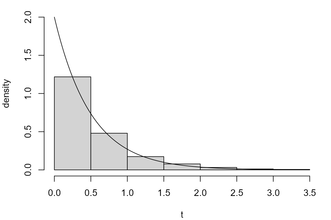

The p.d.f. of an exp(\(\lambda\)) distribution is given by

\[ f_T(t) = \left. \begin{cases} \lambda e^{-\lambda t}, & \text{for } t \geq 0 \\ 0, & \text{for } t < 0. \\ \end{cases} \right. \]

A p.d.f. has the property that it integrates to 1 over the real line and can be used to calculate the probabilities of the form \(P(T \in [a, b])\). In the exponential case, for any \(b > a \geq 0\),

\[ P(T \in [a, b]) = \int_a^b f(t) \mbox{ d}t = \int_a^b \lambda e^{-\lambda t} \mbox{ d}t = e^{-\lambda a} - e^{-\lambda b}. \]

6. Can you guess what the function dexp does? Use ?dexp to find out.

It can be shown that if \(U \sim U(0,1)\) then \(T = -\frac{1}{\lambda} \ln U \sim \mbox{exp}(\lambda)\). This means that we could use the following R code to simulate from an exponential distribution.

u <- runif(1000)
exp_inv <- -log(u)/lambda
par(mar = c(4, 4, 1, 1))
hist(exp_inv, probability = TRUE, ylim = c(0, lambda), main = "", xlab = "t", ylab = "density")
lines(x, dexp(x, rate = lambda))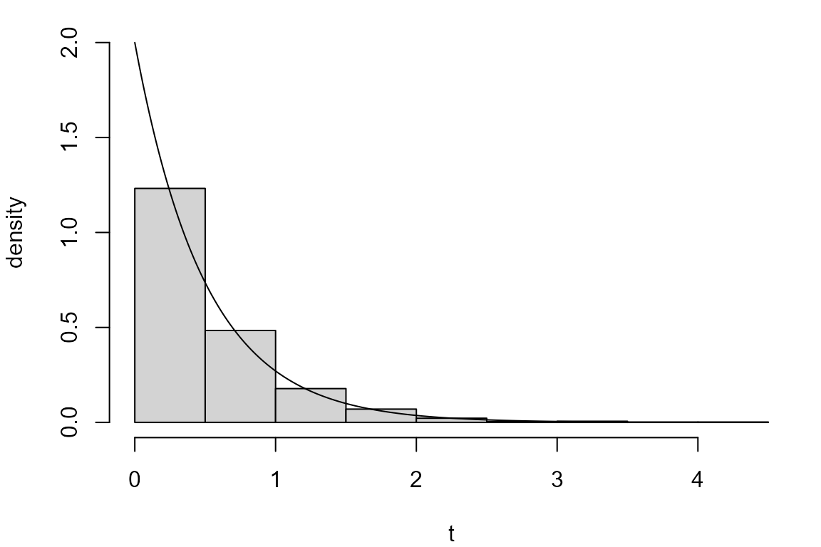

The inversion method

The code immediately above is an example of the inversion method of simulation. The following code implements this for the normal distribution.

u <- runif(1000)
mu <- 0
sigma <- 1
norm_sim <- qnorm(u, mean = mu, sd = sigma)
hist(norm_sim, probability = TRUE, main = "", col = "grey", 
     xlab = "simulated value")
x <- seq(min(norm_sim), max(norm_sim), len = 500)
lines(x, dnorm(x, mean = mu, sd = sigma))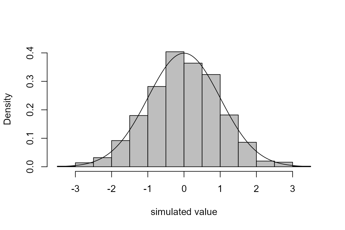

7. Use ?qnorm to find out what qnorm does.

Note that the help page calls this the quantile function. An alternative name is the inverse cumulative distribution function or inverse c.d.f. The c.d.f. of a random variable \(X\) is \(F_X(x) = P(X \leq x)\). We denote the inverse c.d.f. by \(F^{-1}_X(x)\). It can be shown that if \(U \sim U(0,1)\) then \(X = F_X^{-1}(U)\) has c.d.f. \(F_X(x)\), that is, \(X\) has the required distribution.

The inversion method requires us to be able to evaluate quickly the quantile function of the variable in question. This is not always the case. Although it may seem easy to use qnorm to simulate from a normal distribution using the inversion method, calculations using qnorm are not fast and R’s function rnorm uses a more efficient method that avoids using the quantile function. See ?rnorm.

We have illustrated the inversion method using a one-dimensional continuous random variables, the univariate case. The same approach can be used to simulate from the distribution of a discrete random variable and in the multivariate case, that is, the (joint) distribution of a set of two or more related random variables.

Other methods of simulation

Often the most efficient method of simulating values from a probability distribution is one that has been devised for that particular distribution. However, it is useful to have more general methods that can, in principle, be used to simulate from any distribution, although, in practice, there are constraints on the type of distribution to which a method can be applied. Many of these methods work by proposing values and then accepting or rejecting them using a rule, hence they are often called acceptance-rejection or rejection methods. In principle these methods can be used in the \(m\)-dimensional multivariate case but in practice they quickly become inefficient as \(m\) increases.

Example 1. Estimating statistical properties

A commonly-used summary of a random variable its mean, also known as its expectation. For a random variable \(X\), this is denoted \(\mbox{E}(X)\). For a continuous random variable \(X\),

\[ \mbox{E}(X) = \int_{-\infty}^{\infty} x f_X(x) \mbox{ d}x. \]

In simple cases this integral can be evaluated easily, but there are instances where this is not easy. For example, there are cases where the value of p.d.f. \(f_X(x)\) cannot be calculated. If we are able to simulate from the distribution of \(X\) then we can use these simulated values to estimate \(\text{E}(X)\). This technique is called Monte Carlo integration.

Monte Carlo integration

Suppose that \(X \sim U(0,1)\) It can be shown that \(\mbox{E}(X) = 1/2\).

8. Can you provide a non-mathematical argument for this result?

If we simulate a large sample \(x_1, \ldots, x_n\) from a \(U(0,1)\) distribution then we expect its sample mean \[\bar{x} = \frac1n \sum_{i=1}^{n} x_i\] to be close to \(1/2\). The following R code checks this.

u <- runif(10000)
mean(u)
[1] 0.4994436

Hopefully, this seems obvious. There is some theory that supports this idea, the Law of large numbers. Loosely speaking, this means that the estimate of the expectation of the variable provided by the sample mean can be made as precise as we like by increasing the size \(n\) of the simulated sample. In short, the sample mean converges to the expectation as \(n\) tends to infinity. This is illustrated in the following plot.

m <- cumsum(u) / seq_along(u)
plot(seq_along(u), m, type = "l", xlab = "n", ylab = expression(estimate~of~E(X)))
abline(h = 1/2, col = "blue", lty = 2)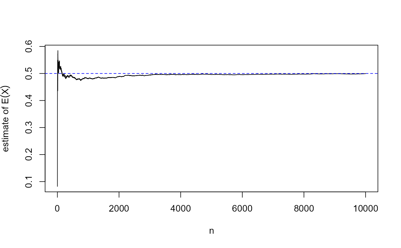

The convergence that we see here is not of a non-random quantity getting inexorably closer and closer to the limit \(1/2\), because as \(n\) increases the estimate can move further from \(1/2\) and then move back towards it. For the so-called weak law of large numbers the idea is that however close to \(1/2\) we require the estimate to be, as \(n\) tends to infinity the probability that our requirement is not satisfied tends to \(0\).

This idea can generalised. Suppose that \(Y\) has p.d.f. \(f_Y(y)\) and instead of \(\mbox{E}(Y)\) we are interested in \(\mbox{E}(g(Y))\) for some function \(g\). \(\mbox{E}(g(Y))\) can be calculated using \[\mbox{E}(g(Y)) = \int_{-\infty}^{\infty} g(y) f_Y(y) \mbox{ d}y.\] If we simulate a sample \(y_1, \ldots, y_n\) from the distribution of \(Y\) then \[\frac1n \sum_{i=1}^{n} g(y_i)\] can be used an as estimate of \(\mbox{E}(g(Y))\).

Estimating \(\pi\) using Monte Carlo integration

You will be familiar with the mathematical constant \(\pi \approx 3.14159\). It can be shown that

\[ \pi = 4 \int_0^1 \sqrt{1 - x ^ 2} \mbox{ d}x = 4 \int_0^1 g(x) f_X(x) \mbox{ d}x, \] where \(g(x) = \sqrt{1 - x ^ 2}\) and \(f_X(x) = 1\) for \(0 \leq x \leq 1\) and \(f(x) = 0\) otherwise.

9. Can you explain why this is true without doing any integration?

\(f_X(x)\) is the p.d.f. of a \(U(0,1)\) random variable. Therefore, \(\pi = 4\,\mbox{E}\left(\sqrt{1 - X ^ 2}\right)\), where \(X \sim U(0,1)\) and if we simulate a sample \(x_1, \ldots, x_n\) from a \(U(0,1)\) distribution then \[\hat{\pi} = \frac4n\sum_{i=1}^n \sqrt{1 - x_i ^ 2}\] is an estimate of \(\pi\) whose precision increases with \(n\).

n <- 1000
x <- runif(n)
y <- sqrt(1 - x ^ 2)
theta <- 4 * cumsum(y) / seq_len(n)
plot(1:n, theta, type = "l", xlab = "n", ylab = expression(estimate~of~pi))
abline(h = pi, col = "blue", lty = 2)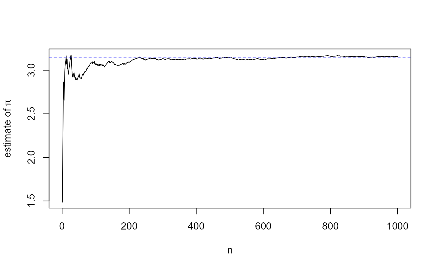

Of course, this isn’t how we would calculate \(\pi\) in practice and when presented with a 1-dimensional integral that we cannot do ‘by hand’, it may be more sensible to use a method of numerical integration, for example the trapezium rule. However, in many statistical problems the \(Y\) in \(\mbox{E}(g(Y))\) is not \(1-\)dimensional but \(m-\)dimensional, where \(m\) is large. For a sufficiently large \(m\), numerical integration techniques may not be effective and Monte Carlo integration may be a better option.

A Monte Carlo estimate of E\((g(Y))\) is a random quantity. Its quality can be measured by its standard deviation, which is of the form \(c /\sqrt{n}\). Tricks can be used to make the value of \(c\) smaller than the simple version described above. If we can simulate effectively from the distribution of \(Y\) (this might not be easy!) and make \(c/\sqrt{n}\) small enough then we can produce a precise estimate.

Example 2. A simple model for an epidemic

Unfortunately, we are well aware of the serious consequences of an outbreak of an infectious disease and the importance of measures to mitigate the effects of such an epidemic. Understanding the way that the infection spreads within a population over time, the dynamics of the epidemic, can help governments to decide which measures to use and when. A common approach is to represent the dynamics using a model, based on a set of assumptions. The model isn’t correct, because it is a simplification of reality. However, if it captures important aspects of the behaviour of the epidemic then it can be useful. In particular, it may be used to answer `What if?’ questions, such as

“What may happen if we implement, or relax, particular public health measures?”.

An SIR model

We consider a very simple epidemic model based on a stochastic process, which is a collection of quantities that vary over time while undergoing random fluctuations. We measure time in days. For simplicity, we assume that everybody recovers from the disease and that people in a population are either:

• susceptible to catching the disease, or
• infected with the disease, or
• recovered from the disease and with life-long immunity to the disease.

After an infected person recovers from the disease they either become immune to the disease, and enter the recovered category, or they do not develop immunity and return to the susceptible category. A model of this general type is called an SIR model.

In describing the assumptions of our model the concept of a Poisson process is important. Informally, in a Poisson process events of interest occur singly, randomly and independently of each other and at a constant rate \(\lambda\) per day. We will observe differing numbers of events on different days, but the mean number \(\lambda\) of events per day is constant over time. A key property of a Poisson process is that if we inspect it at an arbitrarily chosen time then the time until the next event has an exponential(\(\lambda\)) distribution.

Model assumptions

New people enter the population in a Poisson process of rate \(\alpha\) per day.

• Each new person that arrives has a probability \(p_I\) of being infected with the disease.

Each infected person contacts other people in a Poisson process of rate \(\beta\) per day.

• If an infected person contacts a susceptible person then they are infected immediately.

An infected person recovers after a time that has an exponential(\(\gamma\)) distribution, with a mean of \(1/\gamma\).

• When a person recovers the probability that they become immune is \(p_R\).

In addition we assume that each person acts independently of all other people and that the processes governing infection, recovery an the arrival of new people are independent.

It is relatively simple to simulate from this model, so that we can study how an epidemic might evolve over time. We have written an R function rSIR that does this. This function, and technical details that explain how it works, are given in the appendix SIR theory and simulation code

Why simulate from this model?

Even for this simple model important properties may not be obtained easily using mathematics. For example, we may be interested in the probability that demand for treatment for the disease will exceed supply and, if it is exceeded, by how much it will be exceeded and for how long. The answers to the latter questions are not single numbers but probability distributions and these in particular will be difficult to obtain in simple form. The problem will be even more difficult for a more realistic model.

Simulation allows us to answer these questions by simulating from the model, using parameter values that are considered relevant, and calculating quantities of interest based on the simulated data. If we simulate many times then we can estimate the probability that an event happens, using the proportion of simulations in which it happens, and study how important quantities vary between simulations.

Example simulations

The following simulations illustrate the general behaviour of this SIR model an epidemic under this SIR model, using parameter values that are chosen in a fairly arbitrary way. In all cases we consider an initial population size of 1000 people and simulate for a period of 100 days.

What if post-infection immunity is likely?

Firstly, we suppose that initially there is are 10 infected people and the rest of the population is susceptible. We suppose that:

• new people arrive at a rate \(\alpha = 1 / 10\) per day and that \(p_I = 10\%\) of these people are infected
• infected people contact other people at a rate \(\beta = 1\) per day
• on average people remain infected for \(1/\gamma = 5\) days and are then immune with probability \(p_R = 90\%\).

set.seed(31052020)
# parameters: (alpha, pI, beta, pR, gamma)
pars1 <- c(1/10, 0.1, 1, 1/5, 0.9)
I0 <- 10
r1 <- rSIR(pars = pars1, I0 = I0)
par(mar = c(4, 4, 1, 1))
leg <- c("susceptible", "infected", "immune", "population")
matplot(r1[, 1], r1[, -1], type = "l", lty = 1, lwd = 2, col = 1:4, 
        ylab = "number of people", xlab = "time / days")
legend("right", legend = leg, lty = 1, lwd = 2, col = 1:4, bg = "transparent")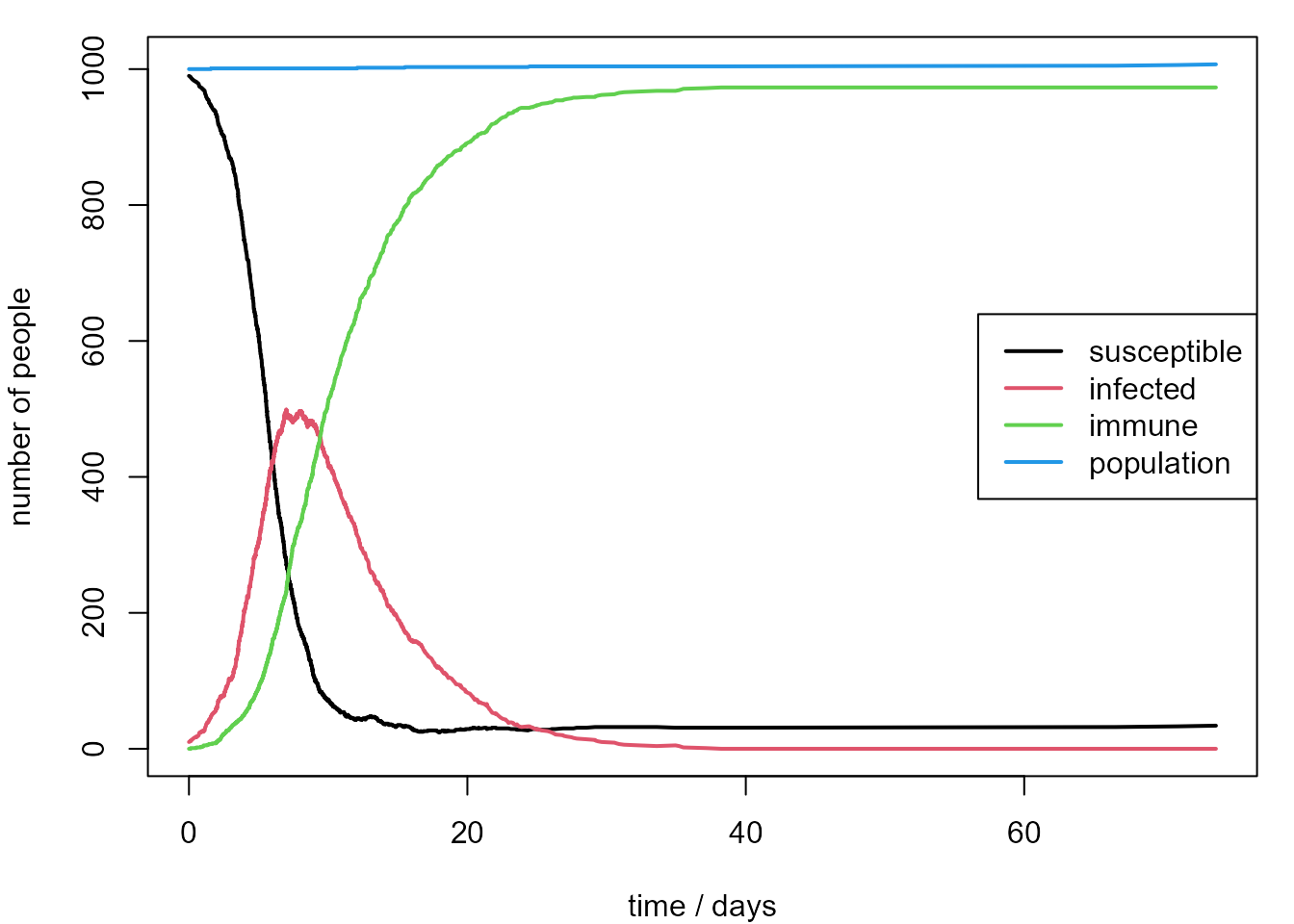

After the infection arrives in the population the number of infected people increases quickly. We expect this because the basic reproduction number \(R_0\) is equal to \(\beta / \gamma = 5\), which is greater than 1. Then the number of infected people drops quickly because many of these people become immune. At the end of 100 days there are still approximately 100 susceptible people in the population. This means that the disease will spread again at some point in the future, but the outbreak may be less dramatic if the proportion of susceptible people in the population is low.

Suppose that we only have resources to treat infected 500 people at any one time. We repeat the simulation from this SIR model 100 times. We plot only the evolution of the number of infected people and calculate the proportion of simulations where the number of infected people exceeds 500 during the 100-day period. This give an estimate of 69% for the probability that our resources are not sufficient.

set.seed(31052020)
r1 <- rSIR(pars = pars1, I0 = I0)
par(mar = c(4, 4, 1, 1))
matplot(r1[, 1], r1[, 3], type = "l", ylab = "number of infected people", 
        xlab = "time / days", ylim = c(0, 550), col = 2)
nsim <- 100
gt500 <- numeric(nsim)
gt500[1] <- any(r1[, 3] > 500)
for (i in 2:nsim) {
  r2 <- rSIR(pars = pars1, I0 = I0)
  matlines(r2[, 1], r2[, 3], col = 2)
  gt500[i] <- any(r2[, 3] > 500)
}
abline(h = 500, lty = 2)
mean(gt500)
[1] 0.69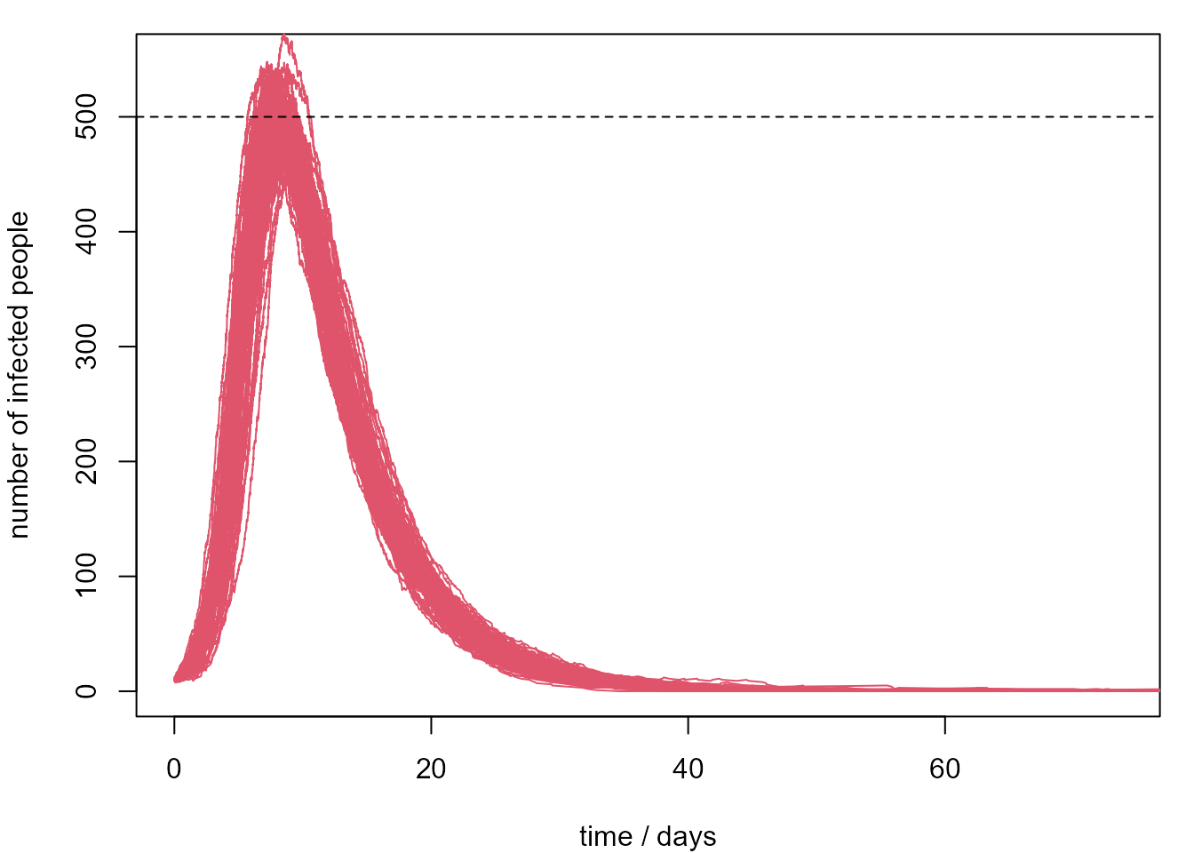

What if post-infection immunity is unlikely?

We re-run the first simulation with the probability \(p_R\) of post-infection immunity set at 10%, rather than 90%. We also extend the simulation to 200 days.

set.seed(31052020)
# parameters: (alpha, pI, beta, pR, gamma)
pars2 <- c(1/10, 0.1, 1, 1/5, 0.1)
r2 <- rSIR(pars = pars2, I0 = I0, days = 200)
par(mar = c(4, 4, 1, 1))
matplot(r2[, 1], r2[, -1], type = "l", lty = 1, lwd = 2, col = 1:4, 
        ylab = "number of people", xlab = "time / days")
legend("right", legend = leg, lty = 1, lwd = 2, col = 1:4, bg = "transparent")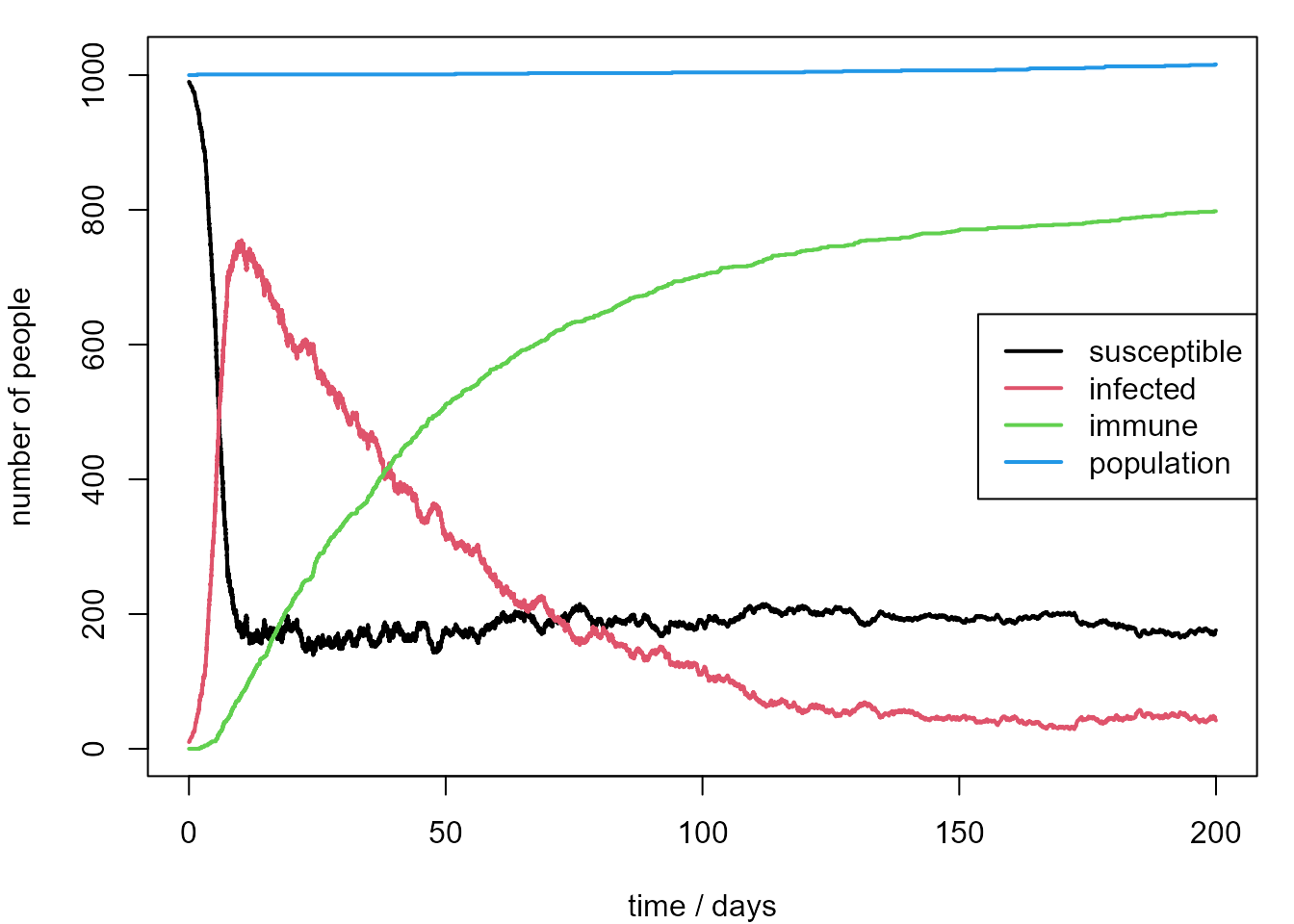

Now the behaviour is rather different. The number of people who are immune rises more slowly than before and the number of infected people drops more slowly after the peak. At the end of 200 days approximately 20% of the population are susceptible to the disease when a new infected person arrives.

Our model is clearly not a useful representation of a COVID-19 outbreak, because it doesn’t reflect the reality of the way that the disease is transmitted and the public health measures used to mitigate its effects. Also the parameter values that we have used have not been informed by expert knowledge or estimated from data.

10. Can you note some ways in which the structure of the models and its assumptions are unrealistic? How might it be made more realistic?

To see some ways in which this kind of model could be extended to increase realism with regard to the COVID-19 outbreak, see Simulating COVID-19 interventions with R. If you read this then you will see that although several simulations are performed only results averaged over these simulations are presented. Studying only the behaviour of averages over time is potentially dangerous, because it this may hide important information about how variable results are over different simulations.

Concluding remarks

I hope that we have convinced you that stochastic simulation is a useful technique and given you some idea how it works. We have presented two examples, but simulation has many more uses. For example, simulation can be used to fit models in cases where it is not possible to perform the mathematics required for more traditional fitting methods. The general idea is that data simulated from a good model for real data should look like the real data, and therefore we should identify combinations of parameters for which this is the case.

Appendix: SIR theory and simulation code

Let \(S(t), I(t)\) and \(R(t)\) denote denote the respective numbers of susceptible, infected and recovered people, and \(N(t) = S(t) + I(t) + R(t)\) the population size, at time \(t\). Let \(X(t) = (S(t), I(t), R(t))\). We start the process at time \(0\), with \(N(0)\) people in the population and \(S(0), I(0)\) and \(R(0)\) people in the three disease categories.

The assumptions of our SIR model are convenient mathematically, that is, they make it easier to study certain properties of the epidemic.
In particular, the following property holds.

The Markov property. If we know the value of \(X(t)\) then the future evolution of the disease does not depend on the numbers of infected, susceptible and recovered people prior to time \(t\).

Simulation from this model

It is easy to simulate from a Markov process, because it breaks down into two separate parts.

1. How long is it until something changes?
2. What kind of a change is it?

It is common to refer to a change as a “jump”. Here, each jump reflects something happening to one person.

For question 1, it doesn’t matter which type of event causes the jump. Suppose that at a time \(t\), \((S(t), I(t)) = (s, i)\). We need to consider the overall rate at which events happen under these conditions. The rate is \(\phi = \alpha + \beta s i / n + \gamma \, i\). The rate of new arrivals is \(\alpha\). The \(\beta s i / n\) term is the overall infection rate, which follows because there are \(i\) people who could infect others and each of their contacts has probability \(s / n\) of being with a susceptible person. The overall recovery rate from the \(i\) infected people is \(\gamma \, i\), because each infected person is recovering at a rate \(\gamma\). Special properties of the exponential distribution mean that the time until the next jump has an exponential distribution, with rate equal to the overall rate.

For question 2, the probability that an event of a particular type is the first event to occur is proportional it rate of occurrence. In fact, the probability that is proportional to it’s rate of occurrence. For question 2 we need also to consider whether or not an arrival is infected and whether or not an infected person becomes immune after recovery.

Simulation from our model

Suppose that \(X(t) = (S(t), I(t), R(t)) = (s, i, r)\).

1. The time until the next jump has an exponential(\(\phi\)) distribution, where \(\phi = \alpha + \beta s i / n + \gamma \, i\).
2. This jump is to
   • \((s, i + 1, r)\) with probability \(\alpha p_I / \phi\) \(~~~~~~~~~~~~~~~~~~~~~~~~~~\)(arrival of an infected person)
   • \((s + 1, i, r)\) with probability \(\alpha (1 - p_I) / \phi\) \(~~~~~~~~~~~~~~~\) (arrival of a susceptible person)
   • \((s, i - 1, r + 1)\) with probability \(\gamma \, p_R i / \phi\) \(~~~~~~~~~~~~~~~~\) (recovery with immunity)
   • \((s + 1, i - 1, r)\) with probability \(\gamma (1 - p_R) i / \phi\) \(~~~~~~\) (recovery with no immunity)
   • \((s - 1, i + 1, r)\) with probability \((\beta s i / n) / \phi\) \(~~~~~~~~~~~\) (infection of a susceptible)

The overall rate \(\alpha\) of arrival splits into a rate of \(\alpha p_I\) for infected arrivals and \(\alpha (1 - p_I)\) of susceptible arrivals. Similarly, the overall recovery rate from the \(i\) infected people is \(\gamma i\), which splits into a rate \(\gamma \, p_R i\) for recovery with immunity and \(\gamma (1 - p_R) i\) for recovery without immunity.

We already how to simulate from an exponential distribution and simulation of the outcome of a jump is a simple extension, from 2 outcomes to 5 outcomes, of the idea that we used when simulating from a binomial distribution.

The Markov property means that when the process jumps, at a time \(t_2 > t\) say, we can just start again with parts 1 and 2. Only the value of \(X(t_2)\) matters, not the history of how this was reached.

The simulation is performed using two R functions. rSIR is the function that we call to set up the simulation. SIRjump is called repeatedly within rSIR: each call simulates the next change, or jump in the state of the process. The arguments (inputs) to the functions are explained in comments at the start. Default values of the arguments are given in the first line of the function. We can change these by specifying different numbers when we use rSIR

rSIR <- function(N0 = 1000, I0 = 0, S0 = N0 - I0, days = 100, 
                 pars = c(1, 0.1, 2, 1, 0.9)) {
  #
  # Simulates from a simple stochastic SIR epidemic model
  #
  # Arguments:
  #   N0     - an integer. The population size at time 0.
  #   I0     - an integer. The initial number of infected people.
  #   S0     - an integer. The initial number of susceptible people.
  #   R0     - an integer. The initial number of recovered people.
  #   days   - an integer. The number of days for which to simulate.
  #   pars   - a numeric vector: (alpha, pI, beta, pR, gamma). 
  #     alpha : rate of arrival of people into the population
  #     pI    : probability that an arrival is infected
  #     beta  : individual infection rate at time t is beta / Nt
  #     gamma : recovery rate for each infected individual
  #     pR    : probability that an infected person is immune after recovery
  #   
  # Returns:
  #   A numeric matrix with 5 columns.  Row i contains the values of 
  #   (t, S_t, I_t, R_t, N_t) immediately after transition i - 1.
  #
  # Checks:
  if (I0 + S0 > N0) {
    stop("There can be at most N people who are susceptible or infected")
  }
  # Infer the number of recovered people
  R0 <- N0 - I0 - S0
  # The initial state, at time = 0
  x <- c(0, S0, I0, R0, N0)
  # A list in which to store the results
  res <- list()
  i <- 1
  # Simulate the next change, or jump, in the process until days have passed
  while (x[1] < days) {
    res[[i]] <- x
    x <- SIRjump(x, pars)
    i <- i + 1
  }
  # Convert the list to a matrix
  res <- do.call(rbind, res)
  colnames(res) <- c("t", "St", "It", "Rt", "Nt")
  return(res)
}

SIRjump <- function (x, pars) {
  #
  # Simulates one jump from a simple stochastic SIS epidemic model
  #
  # Arguments:
  #   x    - a numeric vector: (time, S, I, R, N) at the previous jump.
  #   pars - a numeric vector: (alpha, pI, beta, gamma, pR). 
  #   
  # Returns:
  #   a numeric vector: (time, S, I, R, N) immediately after the next jump  
  #
  # The numbers of susceptible and infected people and the population size
  St <- x[2]
  It <- x[3]
  Rt <- x[4]
  Nt <- x[5]
  # The parameter values
  alpha <- pars[1]
  pI <- pars[2]
  beta <- pars[3]
  gamma <- pars[4]
  pR <- pars[5]
  # Simulate the time at which the next transition occurs
  total_rate <- alpha + beta * St * It / Nt + gamma * It
  x[1] <- x[1] + rexp(1, total_rate)
  # Jump probabilities
  p1 <- alpha * pI / total_rate
  p2 <- alpha * (1 - pI) / total_rate
  p3 <- gamma * pR * It / total_rate
  p4 <- gamma * (1 - pR) * It / total_rate
  u <- runif(1)
  if (u < p1) {
    # Arrival of a new infected person It increases by 1, Nt increases by 1
    x[3] <- x[3] + 1 
    x[5] <- x[5] + 1 
  } else if (u < p1 + p2) {
    # Arrival of a new susceptible person St increases by 1, Nt increases by 1
    x[2] <- x[2] + 1 
    x[5] <- x[5] + 1 
  } else if (u < p1 + p2 + p3) {
    # Infected person becomes immune: It decreases by 1, Rt increases by 1
    x[3] <- x[3] - 1
    x[4] <- x[4] + 1 
  } else if (u < p1 + p2 + p3 + p4) {
    # Infected person becomes susceptible: It decreases by 1, St increases by 1
    x[3] <- x[3] - 1
    x[2] <- x[2] + 1 
  } else {
    # Infection of a susceptible: St decreases by 1, It increases by 1
    x[2] <- x[2] - 1
    x[3] <- x[3] + 1 
  }
  return(x)
}