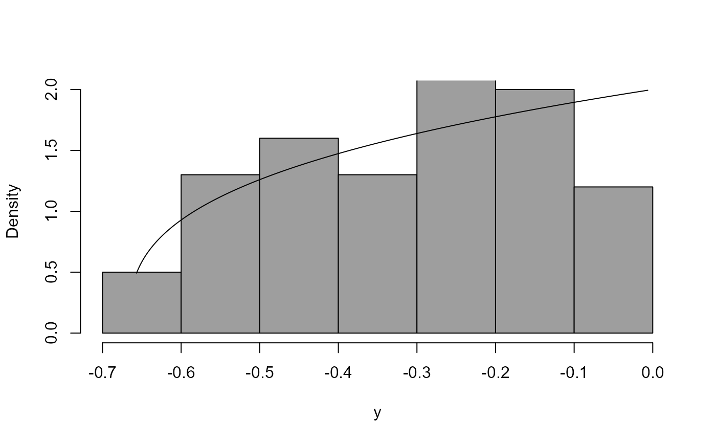
Plot Box-Cox transformed density functions — boxcox

Box-Cox transforms the input data x and plots a histogram of the transformed data. The Box-Cox transformation parameter is lambda. If the probability density function (pdf) from which the data have arisen is known and the function density_fn is supplied to calculate it then this pdf is also Box-Cox transformed and the resulting transformed pdf is superimposed on the histogram.

boxcox_plot(
  x,
  lambda = 1,
  density_fn = NULL,
  breaks = "Sturges",
  main = "",
  ...
)

Arguments

x: A numeric vector of data.
lambda: A numeric scalar. Box-Cox transformation parameter $\lambda$.
density_fn: A function to calculate the pdf underlying the input data.
breaks: The argument breaks of hist. Provided to give control of the appearance of histograms.
main: The argument main of hist. Provided to enable a title to the added to the plot.
...: Further arguments to density_fn (if any).

Value

Nothing, just the plot.

Details

The equation $$y = (x ^ \lambda - 1) / \lambda.$$ is a Box-Cox transformation of a variable $x$ to produce a transformed variable variable $y$. The value of the parameter $\lambda$ governs the behaviour of the transformation.

See the vignette Chapter 2: Graphs (More Than One Variable) for more details of what the code in Examples below is doing.

Examples

# Log-normal distribution --------------------

# X has a log-normal distribution if ln(X) has a normal distribution

# Simulate a sample of size 100 from a log-normal distribution
x <- rlnorm(100)

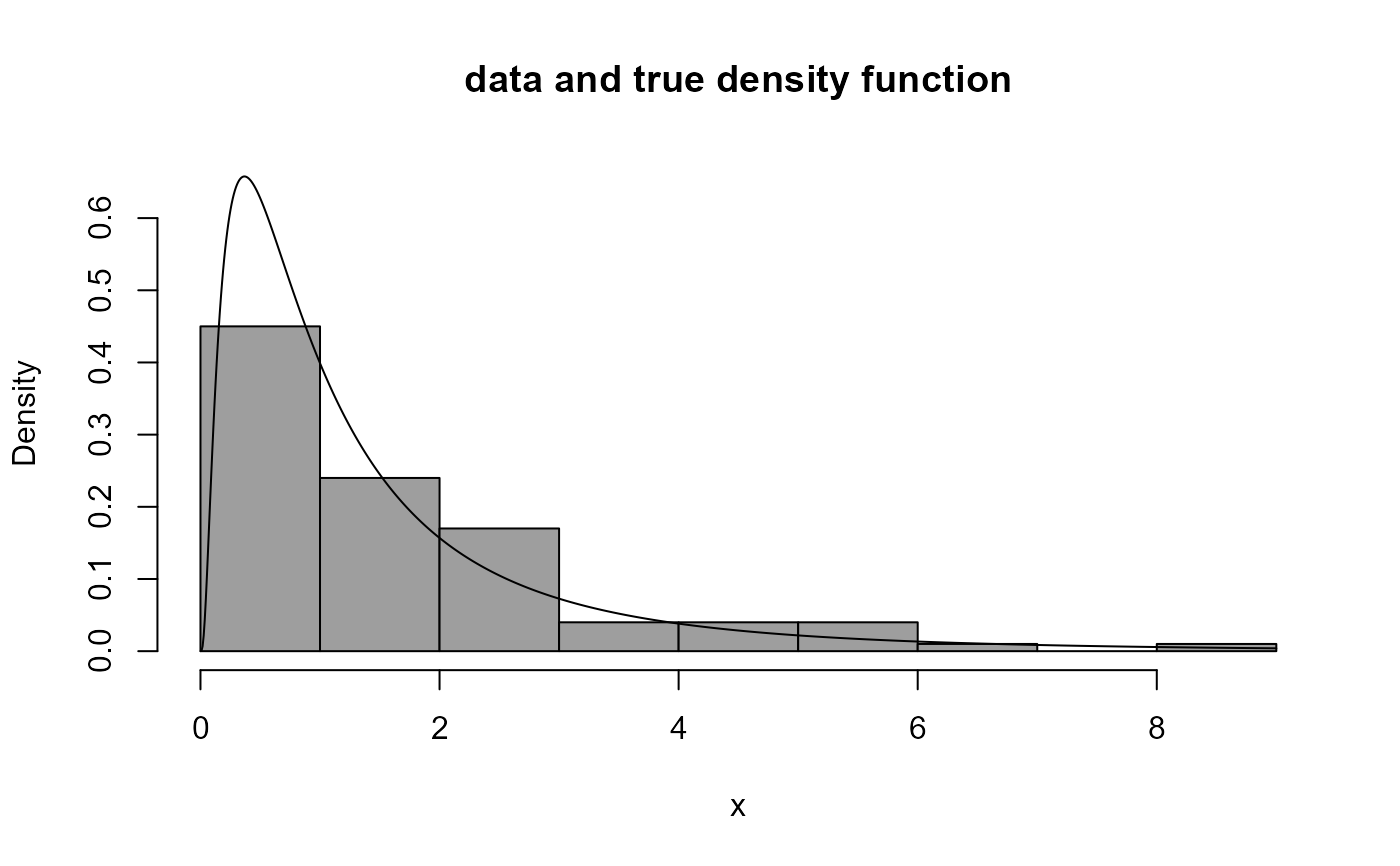
# Plot the data and the log-normal density function
boxcox_plot(x, density_fn = dlnorm, main = "data and true density function")

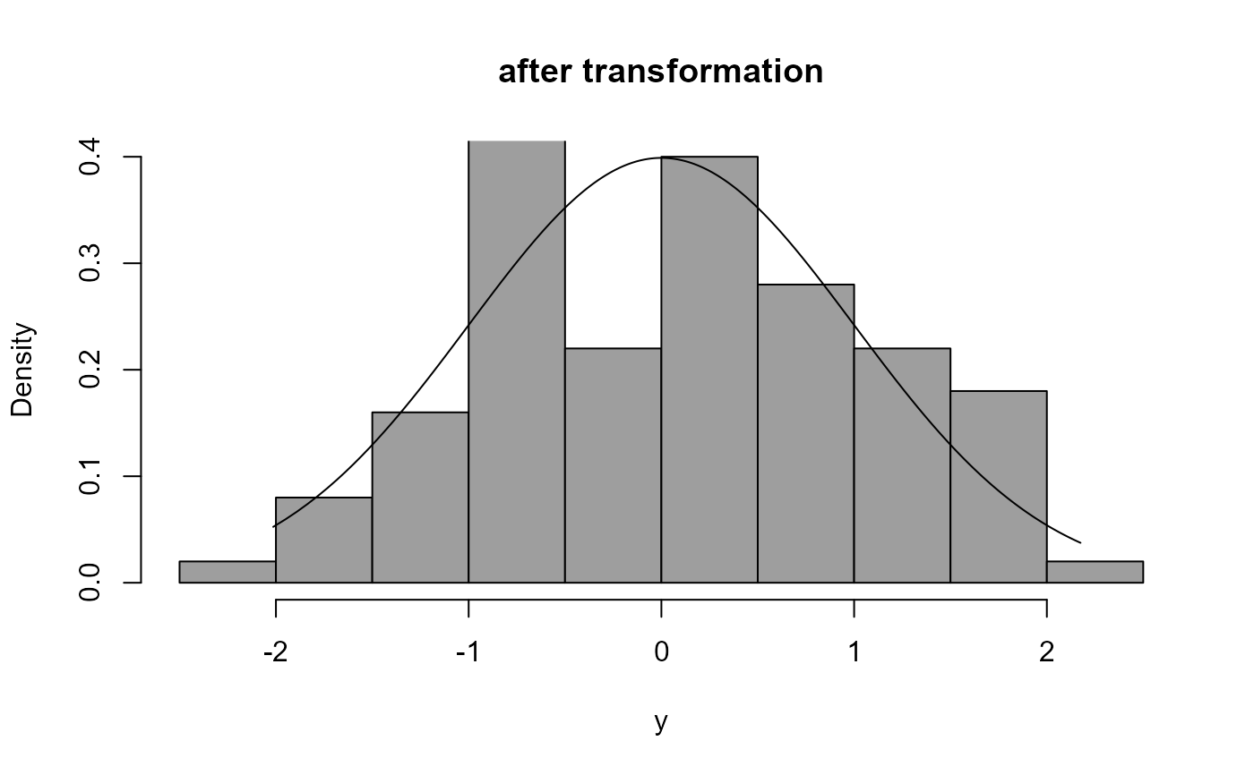
# If we want to transform to approximate normality which power should we use?
boxcox_plot(x, density_fn = dlnorm, lambda = 0, main = "after transformation")


# We can use the data to suggest a good value of lambda.
# We need the boxcox() function in the MASS package.
library(MASS)
#> 
#> Attaching package: 'MASS'
#> The following object is masked from 'package:stat0002':
#> 
#>     shuttle

# Very loosely speaking ...
# In this plot better values of lambda have the largest values.
# "Better" means "transformed data closer to looking like a sample
# from a normal distribution.
# We could choose a nice value of lambda close to the best value.
# The interval is a 95% confidence interval for lambda.
boxcox(x ~ 1)


# exponential distribution --------------------

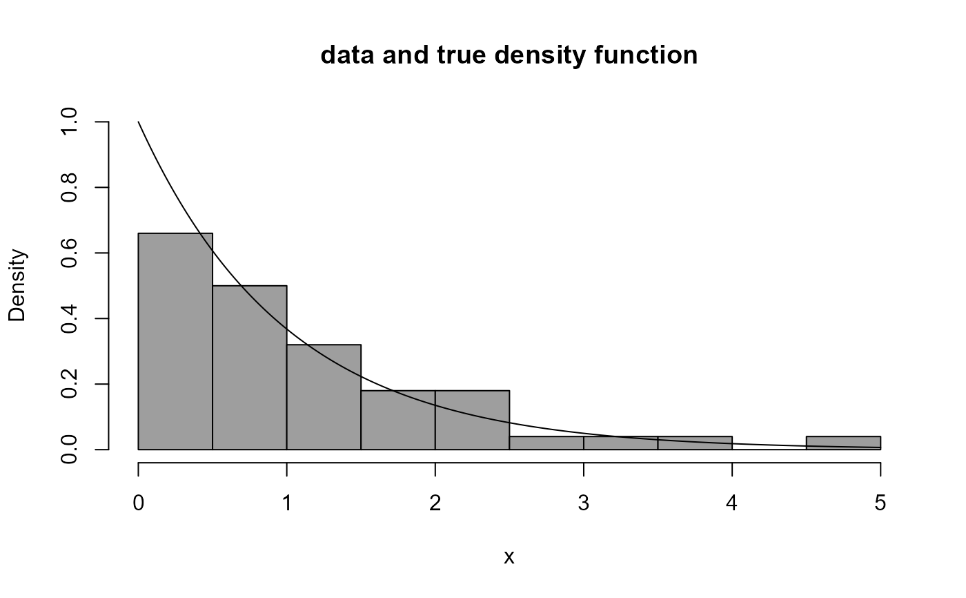
x2 <- rexp(100)
boxcox_plot(x2 ,density_fn = dexp, main = "data and true density function")


boxcox_plot(x2, density_fn = dexp, lambda = 1 / 3, main = "after transformation")

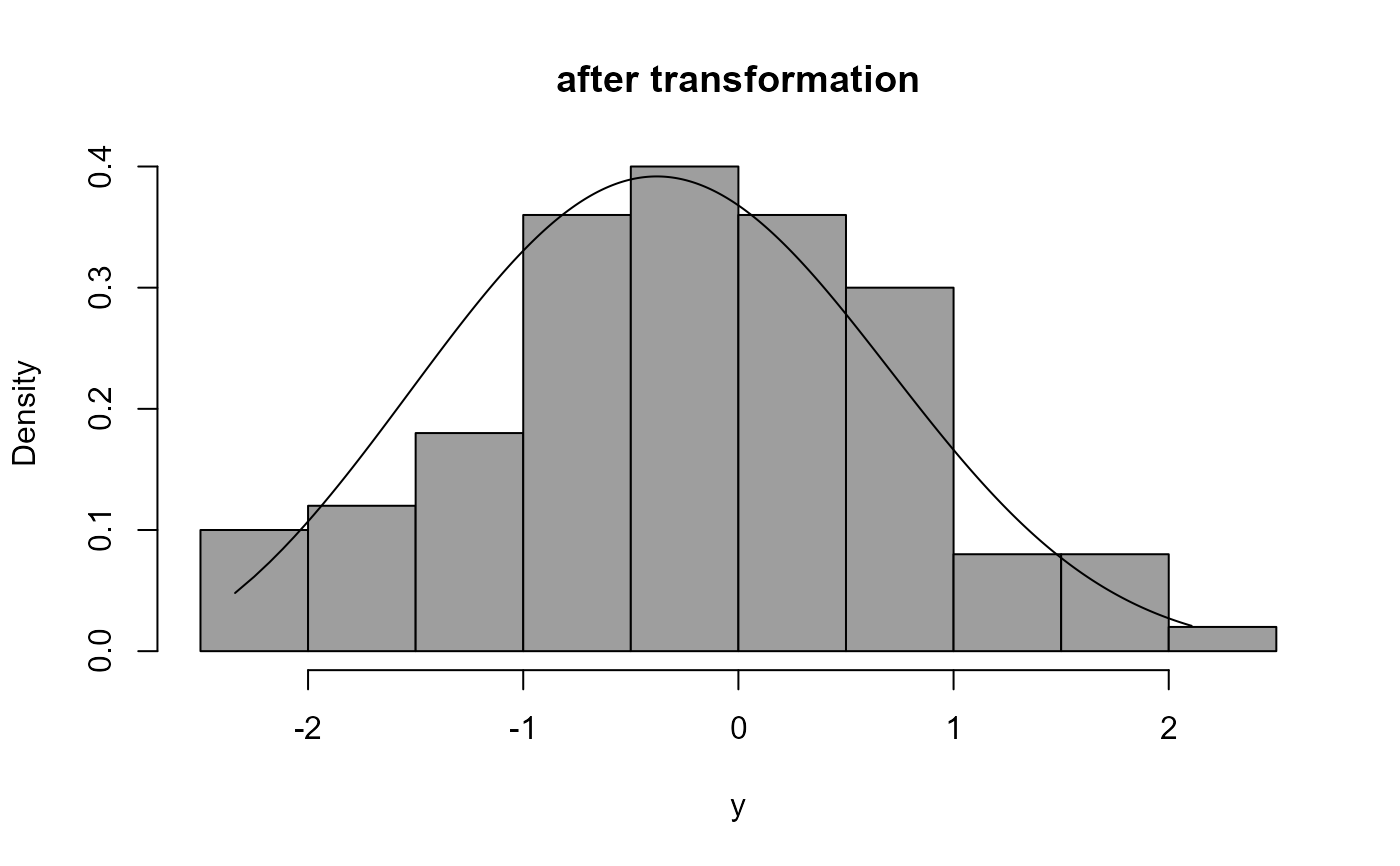boxcox(x2 ~ 1)
abline(v = 1/3, col = "red")


# A distribution that I made up --------------------

dpn <- function(x) ifelse(x > 0 & x < 1, 2 * x, 0)
rpn <- function(n = 1) sqrt(runif(n))
x3 <- rpn(100)
boxcox_plot(x3, density_fn = dpn)

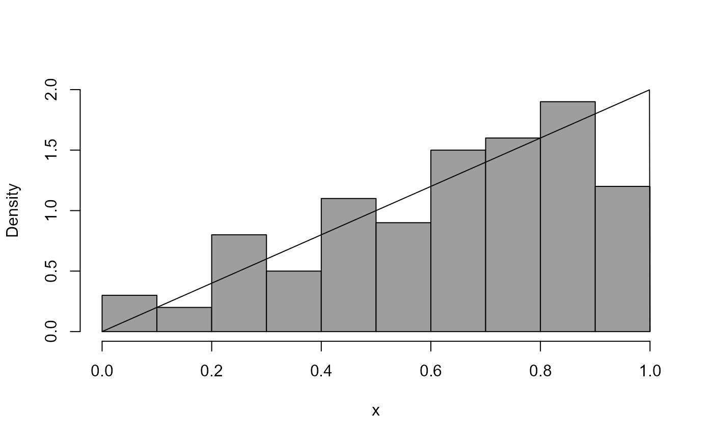boxcox_plot(x3, density_fn = dpn, lambda = 2)


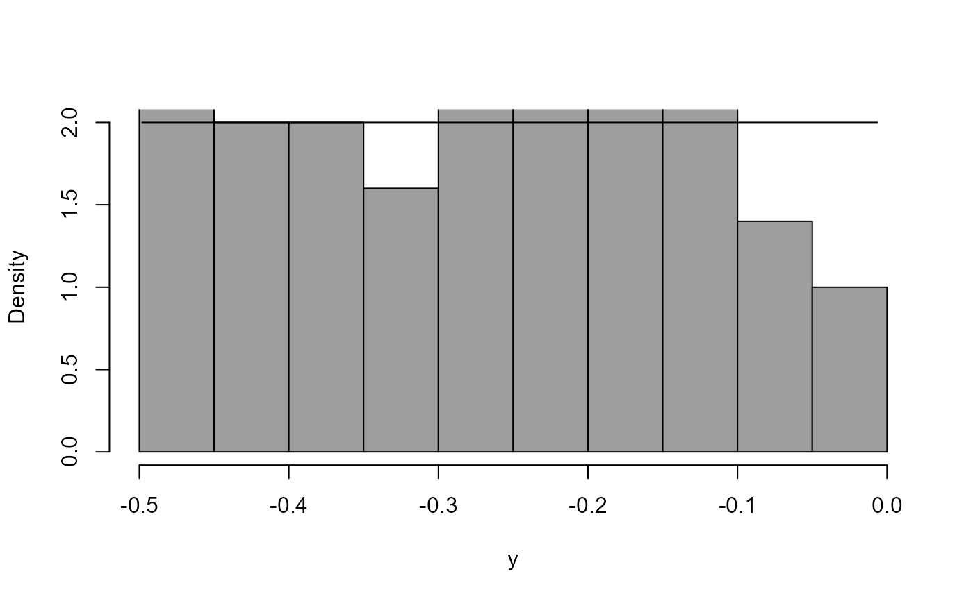boxcox(x3 ~ 1)

boxcox(x3 ~ 1, lambda = seq(0, 4, 1 / 10))

boxcox_plot(x3, density_fn = dpn, lambda = 1.5)