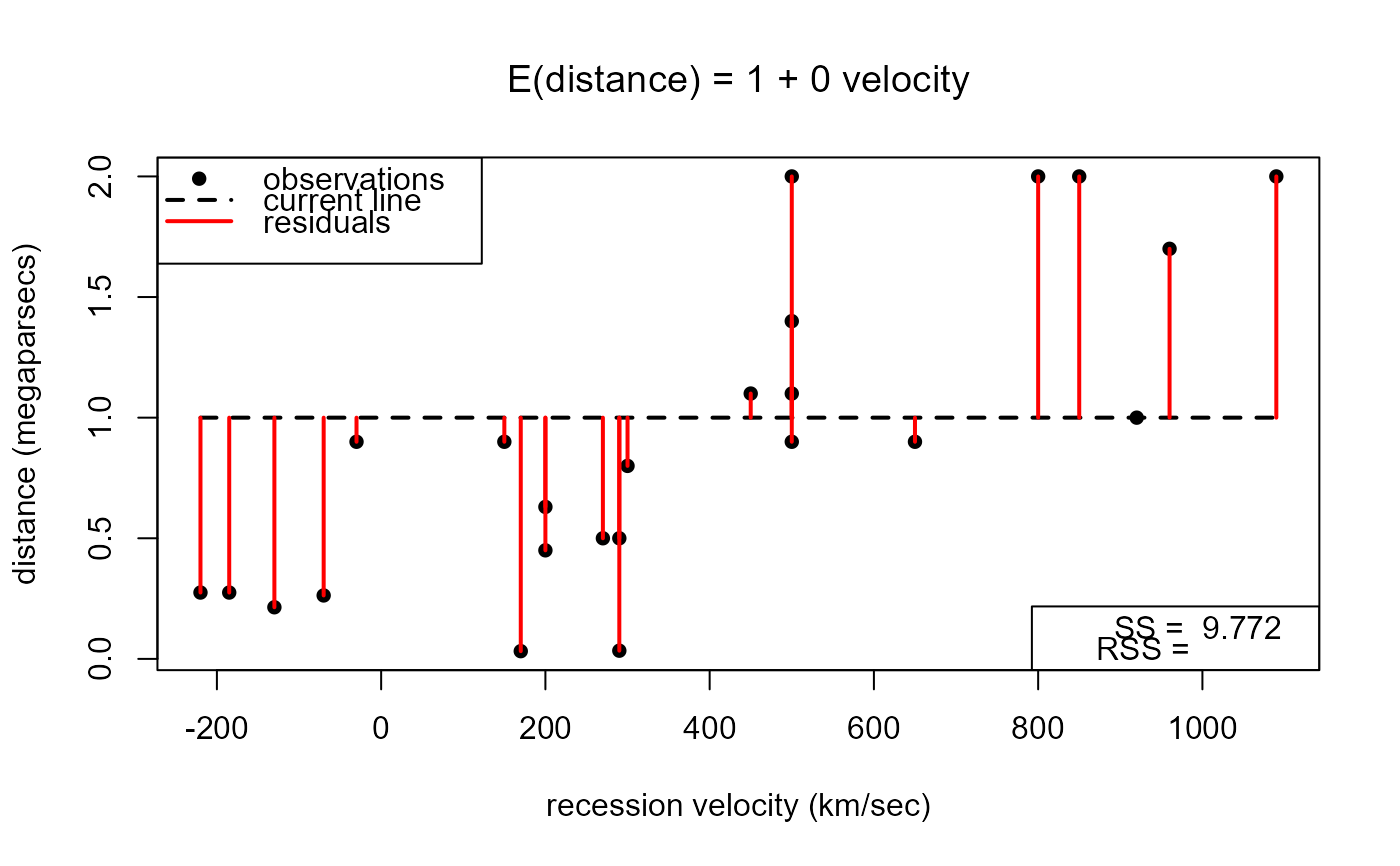
A movie to help to visualize the fitting of a regression line using least squares in the case of a simple linear regression, that is, a linear regression of one response variable on one explanatory variable.
Arguments
- data
A data frame with two variables or a numeric matrix with 2 columns. The first column must contain the response data, the second column the explanatory data.
- delta_alpha, delta_beta
Numeric scalars. The respective amounts by which the values of the intercept and gradient of the line are increased/decreased after one click of the +/- button. The default values are set with the
hubbledata used in the example below in mind.- ...
Further arguments, such as graphical parameters (see
parto be passed toplotwhen producing a scatter plot of the response data against the explanatory data. For example, the plotting character used for the points can be chosen usingpch. Ifpchhas length greater than 1 then only the first element is used. The default value ofpchis 16 (filled circle). The labels on the horizontal and vertical axes can be specified usingxlabandylabrespectively.
Details
A scatter plot of response data against the explanatory data is produced. On this plot is superimposed a dashed line that the user can move, by changing its intercept alpha and gradient beta using +/- buttons. The initial value of alpha is the mean of the response data and the initial value of beta is 0. The sizes of the residuals are shown using red lines. One of the legends gives the current sum of squares residuals (SS).
Another +/- button allows the user to add the least squares regression line to the plot, and the associated residual sum of squares (RSS) to the legend, for comparison.
See also
stat0002movies: general information about the movies.
