Produces a QQ plot to compare ordered sample data to corresponding quantiles of an exponential distribution fitted to these data.
Arguments
- y
Sample data
- statistic
A character scalar. Selects the summary statistic used to estimate \(\lambda\), either the sample mean or sample median.
- type
An integer scalar. If
statistic = "median"then this is passed toquantileto select the type of sample quantile used to estimate the sample median. The default,type = 6, selects the estimator defined in the STAT002 notes.- envelopes
Determines whether or not simulation envelopes should be added to the plot. If
envelopes = FALSEthen no envelopes are added. Ifenvelopesis a positive integer (a common choice is 19) then simulation envelopes based on this many simulated datasets are added. The limits of of the envelopes are indicated using short horizontal lines.- ...
Optional arguments to be passed to
plotsuch asxlab,ylab,mainand/orgraphical parameterssuch aspch,ltyandlwd, to control the appearance of the main plot. To change the appearance of the line of equality use the argumentline.- line
Determines whether or not a line of equality is superimposed on the plot. If a line is required then must be a list, which can contain
graphical parameterspassed toabline, such ascol,ltyandlwdto control the appearance of the line. Iflineis not a list, for example,line = 0, then no line is superimposed.
Details
The rate parameter \(\lambda\) of the exponential distribution
is estimated using 1/mean(y, na.rm = TRUE) if
statistic = "mean" and
log(2)/quantile(y, probs = 0.5, na.rm = TRUE) if
statistic = "median". The ordered sample data are plotted against
quantiles of this fitted exponential distribution. Specifically, the
\(i\)th smallest sample observation is plotted against the
\(100 i / (n + 1)\%\) theoretical exponential quantile, where \(n\) is
the sample size. The plot is constrained to be square. A line of equality
is superimposed on the plot.
See also
qqnorm to produce a normal QQ plot.
Examples
## Australian Birth Times Data
# Calculate the waiting times until each birth
waits <- diff(c(0, aussie_births[, "time"]))
# Estimating lambda using the sample mean
qqexp(waits)
 #> estimate of lambda
#> 0.03066202
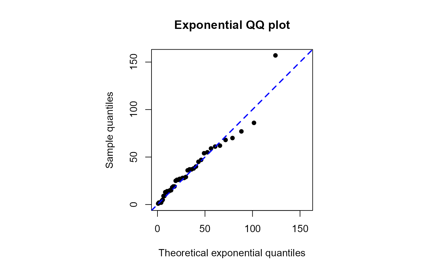
# Change the appearance of the points and line
qqexp(waits, pch = 16, line = list(lty = 2, col = "blue", lwd = 2))
#> estimate of lambda
#> 0.03066202
# Change the appearance of the points and line
qqexp(waits, pch = 16, line = list(lty = 2, col = "blue", lwd = 2))
 #> estimate of lambda
#> 0.03066202
# Add simulation envelopes
qqexp(waits, envelopes = 19)
#> estimate of lambda
#> 0.03066202
# Add simulation envelopes
qqexp(waits, envelopes = 19)
 #> estimate of lambda
#> 0.03066202
# Estimating lambda using the sample median
qqexp(waits, statistic = "median", envelopes = 19)
#> estimate of lambda
#> 0.03066202
# Estimating lambda using the sample median
qqexp(waits, statistic = "median", envelopes = 19)
 #> estimate of lambda
#> 0.0261565
#> estimate of lambda
#> 0.0261565