Chapter 8 Contingency tables

In this chapter, and the next chapter on linear regression, we explore the relationships between two, or more, variables. In this chapter we consider the situation where all variables are categorical. In Chapter 9 the main variable of interest is continuous.

Suppose that for each of a number of objects/people/experimental units we record the value of 2 of more categorical variables. For each variable the categories must be mutually exclusive and exhaustive. For example, in the Berkeley admissions data for each applicant we record the sex (Male/Female) and the outcome of the application (Accept/Reject). We present these data in a contingency table, which summarises the number (frequency or count) of subjects falling into each of the possible categories defined by the categorical variables. A contingency is an event that may occur a possibility. A contingency table is a summary of the frequencies with which combinations of such events occur.

The main aim of analysing data in a contingency table is to examine whether the values of the categorical variables are associated with each other, and, if they are associated, how they are associated. In other words, we ask the question: “How does the distribution of one variable depend on the value of the other variable?”.

Note that association does not imply causation. Just because two variables are associated it does not mean that one variable affects (causes) the other directly. It may be that the association between the two variables is due to each of their relationships with another variable. This seems to be the case for the Berkeley admissions data. We will consider 2-way contingency tables - where subjects are classified according to 2 categorical variables - and 3-way contingency table - where they are classified according to 3 categorical variables.

We return to the Berkeley admissions data. We have already seen the 2-way contingency table in Figure 8.1.

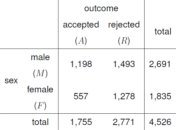
Figure 8.1: 2-way contingency table for the Berkeley admissions data.

This is a 2 \(\times\) 2 (or 2 by 2), contingency table: there are 2 row categories (\(M\) and \(F\)) and 2 column categories (\(A\) and \(R\)). The 4 squares in the middle of the table are called the cells. The sums of the numbers in the cells across the rows are called the row totals. For these data the row totals 2691 and 1835. Similarly, the column totals are 1755 and 2771.

These Berkeley admissions data also contain the department to which the applicants applied. We include this information to extend the 2-way contingency table in Figure 8.1 to produce the 3-way contingency table in Figure 8.9 at the start of Section 8.2.

In Chapter 3 we defined the population of interest to be graduate applications to Berkeley in 1973. We calculated, for example, the probability that an applicant chosen at random from this population is accepted. Now we will be more adventurous. We are interested in graduate applications to Berkeley in general. We wish to make inferences about the probabilities of acceptance for males and females, generally, not just those who happened to apply in 1973. The applications from 1973 are merely a (hopefully representative) sample of data which we use to make inferences about these probabilities. We wish to examine whether sex and the outcome of the application are associated. We do this in Section 8.1. We also wish to consider how the department to which the applicant applies affects things. We do this in Section 8.2. We will see that when there are more than two variables there are several ways to study the association between them.

8.1 2-way contingency tables

We analyse the data in Figure 8.1. We will consider two questions.

Question 1: independence. Are the random variables outcome and sex independent?

Question 2: comparing probabilities. Is the probability of acceptance equal for males and females?

These questions are very similar, but there is a subtle distinction between them. Question 1 treats both outcome and sex as random variables. In Question 2 we condition on the sex of the applicant and compare the probabilities of acceptance that we obtain in each case.

We will see that the calculations performed to answer Question 1 are the same as those performed to answer Question 2. Therefore, you may wonder why we bother to make this distinction. The reason is that there are situations where it is not appropriate to treat both variables as random variables. There are contingency tables where some of the totals are are fixed in advance before the data are collected. For example, it may be that the row totals are known in advance. In the current context, this would mean that Berkeley decided in advance to consider exactly 2691 applications from males and 1835 applications from females. In that event we cannot treat sex as a random variable, because the numbers of males and females is not random.

This is clearly not what would have happened in this example. Nevertheless, we consider both questions because there are examples where totals are fixed. An example is a case-control study, in which potential risk factors for a disease are studied by looking for differences in characteristics between people who have the disease, the cases, and those who do not, the controls. We return to this in Section 8.1.3.

8.1.1 Independence

Question 1: independence. Are the random variables outcome and sex independent?

In the Berkeley example we have two categorical random variables; sex (2 levels: \(M\) and \(F\)) and outcome (2 levels: \(A\) and \(R\)). We wish to examine whether the categorical random variables sex (rows of the table) and outcome (columns of the table) are independent. To do this we compare the observed frequencies with the frequencies we expect if the random variables sex and outcome are independent.

How can we estimate the expected frequencies? If the random variables sex and outcome are independent then \[ P(M, A) = P(M)P(A), \quad P(F, A)=P(F)P(A), \] \[ P(M, R) = P(M)P(R), \quad P(F, R)=P(F)P(R). \]

To get the expected frequencies we multiply these probabilities by 4526. We do not know these probabilities. Therefore, we estimate them using proportions in the observed data: \[ \hat{P}(M)=\frac{2691}{4526}, \,\, \hat{P}(F)=\frac{1835}{4526}, \,\, \hat{P}(A)=\frac{1755}{4526}, \,\, \hat{P}(R)=\frac{2771}{4526}. \]

Therefore, the expected frequency for sex=\(M\) and outcome=\(A\) is estimated as \[ \frac{2691}{4526} \times \frac{1755}{4526} \times 4526 = \frac{2691 \times 1755}{4526} = 1,043.46. \]

The other expected frequencies are estimated similarly to give Figure 8.2.

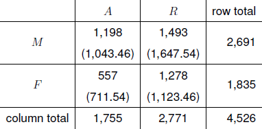
Figure 8.2: Observed frequencies and estimated expected frequencies (in brackets) under independence of sex and outcome.

Note that the row totals of the estimated expected frequencies are equal to the observed row totals, and similarly for the column totals. In other words the estimated expected frequencies preserve the row and column totals.

We can see that more males are accepted than expected (1,198 accepted compared to the 1,043.5 expected) and fewer females are accepted than expected (557 accepted compared to the 711.5 expected). The fact that the observed frequencies are different from the estimated expected frequencies does not mean that sex and outcome are dependent. However, if the observed and estimated expected frequencies are very different then we might doubt that sex and outcome are independent.

Notation

We define some general notation for use with an \(I \times J\) contingency tables. Let

• \(X\) be the random variable on the rows of the table. (\(X=1,2,\ldots, I-1\) or \(I\)).
• \(Y\) be the random variable on the columns of the table. (\(Y=1,2,\ldots, J-1\) or \(J\)).
• \(n_{ij}\) be the observed frequency for the event \(\{X=i\) and \(Y=j\}\).
• \(n_{i+}=\displaystyle\sum_{j=1}^J n_{ij}\), the sum of the frequencies in row \(i\).
• \(n_{+j}=\displaystyle\sum_{i=1}^I n_{ij}\), the sum of the frequencies in column \(j\).
• \(n\) be the sample size.

Figure 8.3 illustrates this notation.

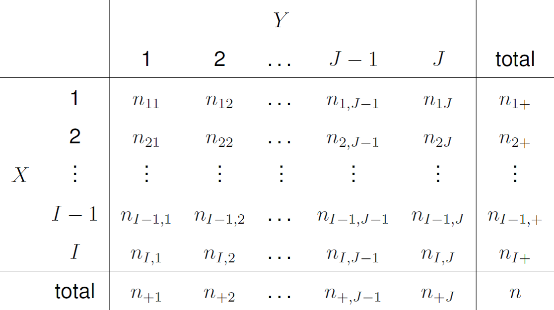
Figure 8.3: Notation for a 2-way contingency table.

Calculating estimated expected frequencies under independence

For \(i=1,\ldots,I\) and \(j=1,\ldots,J\) the observed frequency \(n_{ij}\) is the sample value of a random variable \(N_{ij}\) with expected value \(\mu_{ij}\).

Let \[ p_{ij} = P(X=i, Y=j) \] and \[ p_{i+}=\displaystyle\sum_{j=1}^J p_{ij}=P(X=i) \quad \mbox{and} \quad p_{+j}=\displaystyle\sum_{i=1}^I p_{ij}=P(Y=j). \]

\[ p_{i+} \mbox{ is the probability of being in row }i \]

\[ p_{+j} \mbox{ is the probability of being in column }j \]

If \(X\) and \(Y\) are independent then

\[ p_{ij} = P(X=i, Y=j) = P(X=i)\,P(Y=j) = p_{i+}\,p_{+j}. \]

Therefore the expected frequency for the \((i,j)\)th cell in the table is given by

\[ \mu_{ij} = n\,p_{ij} = n\,p_{i+}\,p_{+j}. \]

We estimate \(p_{i+}\) and \(p_{+j}\) using

\[ \hat{p}_{i+} = \frac{n_{i+}}{n}, \quad \mbox{and} \quad \hat{p}_{+j} = \frac{n_{+j}}{n}, \]

to give the estimated expected frequency

\[ \hat{\mu}_{ij} = n\,\hat{p}_{i+}\,\hat{p}_{+j} = n\,\frac{n_{i+}}{n}\,\frac{n_{+j}}{n} = \frac{n_{i+}\,n_{+j}}{n}. \]

Residuals

To help us compare the observed and estimated expected frequencies we can use residuals. We define, for \(i=1,\ldots,I,\,j=1,\ldots,J\), (estimated) residuals: \[ r_{ij} = n_{ij}-\hat{\mu}_{ij}. \] However, the residuals will tend to be larger for cells with larger estimated expected frequencies. Instead we can use Pearson residuals \[ r^P_{ij} = \frac{n_{ij}-\hat{\mu}_{ij}}{\sqrt{\hat{\mu}_{ij}}}, \] or standardised Pearson residuals \[ r^{S}_{ij} = \frac{n_{ij}-\hat{\mu}_{ij}}{\sqrt{\hat{\mu}_{ij}\, \left(1-\hat{p}_{i+}\right)\,\left(1-\hat{p}_{+j}\right)}}. \]

Example calculation of residuals for cell (1,1)

\[ \hat{p}_{1+} = \frac{2691}{4526} = 0.59, \qquad \hat{p}_{+1}=\frac{1755}{4526} = 0.39. \]

\[ \hat{\mu}_{11} = \frac{n_{1+}\,n_{+1}}{n} = \frac{2691 \times 1755}{4526} = 1043.46. \]

\[ r_{11} = n_{11}-\hat{\mu}_{11} = 1198 - 1043.46 = 154.54. \]

\[ r_{11}^P = \frac{r_{11}}{\sqrt{\hat{\mu}_{11}}} = \frac{154.54}{\sqrt{1043.46}} = 4.78. \]

\[ r_{11}^S = \frac{r_{11}^P}{\sqrt{(1-\hat{p}_{1+})\,(1-\hat{p}_{+1})}} = \frac{4.78}{\sqrt{\left(1-\displaystyle\frac{2691}{4526}\right)\,\left(1-\displaystyle\frac{1755}{4526}\right)}}=9.60. \]

We have found that the observed frequencies are different to those expected if outcome and sex are independent, producing non-zero residuals. Even if outcome and sex are independent it is very unlikely that the residuals will be exactly zero. The question is whether these residuals are so large to suggest that outcome and sex are not independent. To assess this we need to know what kind of residuals tend to occur when outcome and sex are independent. If residuals that are as large or larger then the ones that we have observed are unlikely to occur then it suggests that outcome and sex are not independent.

If \(X\) and \(Y\) are independent, and if the expected frequencies are large enough (a check is that all the estimated expected frequencies are greater than 5), each Pearson residual, and each standardised Pearson residual, has approximately a normal distribution with mean 0. In addition the standardised Pearson residuals have an approximate variance of 1. So, if these assumptions are true, the standardised Pearson residuals are approximately N(0,1). Owing to the properties of the N(0,1) distribution, most (approximately 95%) of the residuals should lie in the range \((-2, 2)\). The presence of residuals that have a large magnitude would be surprising and may suggest that \(X\) and \(Y\) are not independent.

The residuals, Pearson residuals and standarised Pearson residuals for the Berkeley admissions example are given in Figure 8.4. The residuals show that approximately 155 more males, and 155 fewer females, are accepted than expected. The standardised Pearson residuals are much larger in magnitude than 2 suggesting that outcome is not independent of sex. This may seem like a very informal way to make an assessment, but we will see that in this case this is equivalent to a more formal-looking approach based on an hypothesis test.

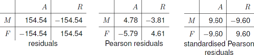
Figure 8.4: Residuals, Pearson residuals and standardised Pearson residuals for the 2-way Berkeley admissions contingency table.

Notice that the residuals are equal in magnitude - so really there is only one residual. The row sums and the column sums of the residuals are equal to zero because the estimated expected frequencies preserve the row and column totals. The residuals have this property for all \(I \times J\) contingency tables. In the \(2 \times 2\) case this means that only 1 of the estimated expected frequencies is free to vary, in the sense that it we calculate one of the estimated expected frequencies then the values of the other 3 estimated expected frequencies follow directly from the fact that the residuals sum to 0 across the rows and down the columns. We say that there is only 1 degree of freedom. This is why, if we perform an hypothesis like the one outlined below, the test statistic is related to the distribution of a chi-squared distribution with 1 degree of freedom.

Things are not so simple for standardised Pearson residuals, but it is true that the sums of the standardised Pearson residuals over a variable will be equal to zero if that variable has two levels. In this \(2 \times 2\) case both the row sums and column sums of the standardised Pearson residuals are equal to zero.

Now we assess whether outcome and sex are independent in a more formal way, using an hypothesis test.

A brief outline of hypothesis testing in this case

General idea:

• assume that sex and outcome are independent (null hypothesis \(H_0\));
• calculate the expected frequencies assuming that sex and income are independent;
• compare the observed frequencies with the expected frequencies;
• assess whether the observed and expected counts are so different that they suggest that sex and outcome are not independent. Above we used standardised residuals to help us assess this.

This is an outline of an hypothesis test. You will see that the test is based on \[ X^2 = \sum_{i,j} \left(r_{ij}^P\right)^2 = \sum_{i,j} \frac{\left(n_{ij}-\hat{\mu}_{ij}\right)^2}{\hat{\mu}_{ij}}, \] which combines the Pearson residuals into a single value.

It can be shown that if the null hypothesis \(H_0\) is true (and the expected frequencies are sufficiently large: again we check that the estimated expected frequencies are greater than 5) then, before we have observed the data, the random variable \(X^2\) has (approximately) a chi-squared distribution with 1 degree of freedom, denoted \(\chi^2_1\).

To demonstrate that this is the case we use simulation. We simulate 1000 2 \(\times\) 2 tables of data, like those in Figure 8.1 except that the data have been simulated assuming that outcome and sex are independent. Figure 8.5 is a histogram of the resulting 1000 values of the \(X^2\) statistic. Also shown is the p.d.f. of a \(\chi^2_1\) random variable.

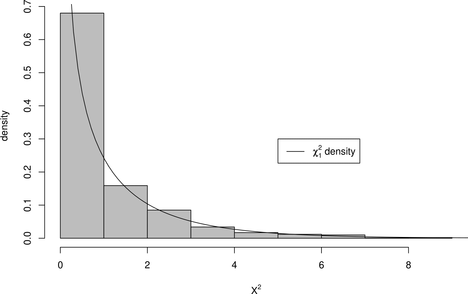
Figure 8.5: Histogram of the \(X^2\) statistic values from 1000 simulated 2 \(\times\) 2 contingency tables, where the row and column variables are independent.

We can see that values of \(X^2\) above 4 are rare. It can be shown that, under \(H_0\) a value above 3.84 will only occur 5% of the time. The value of \(X^2\) from the real data is 92.21. Clearly a value as large as this is very unlikely to occur if \(H_0\) is true. In fact, the probability (a \(p\)-value) of observing a value of \(X^2\) greater than 92.21 is less than \(2.2 \times 10^{-16}\). A \(p\)-value is a measure of our surprise at seeing the data we observe if \(H_0\) is true. This very small \(p\)-value suggests that \(H_0\) is not true, so we would reject \(H_0\).

It is not a coincidence that the square root of the \(X^2\) statistic, \(\sqrt{92.21}\), is equal to \(9.60\), the magnitude of the standardised Pearson residual. In the \(2 \times 2\) case assessing the magnitude of the standard Pearson residuals is equivalent to performing the hypothesis test based on the \(X^2\) statistic.

Now suppose that the real data had given a value of 0.45, for example. The histogram suggests that under \(H_0\) a value as large as this is quite likely to occur (in fact 0.45 is the median of the \(\chi^2_1\) distribution) so we would not reject \(H_0\).

8.1.2 Comparing probabilities

Question 2: comparing probabilities. Is the probability of acceptance equal for males and females?

Now suppose that Berkeley used method 3 to collect the data. If this is the case we cannot estimate \(P(M)\) (or \(P(F)\)), or joint probabilities such as \(P(M, A)\). It is not meaningful to ask whether sex and outcome are independent because sex is not a random variable; the proportions of males and females have been fixed in advance by Berkeley.

However, it is meaningful to look at the conditional distribution of the random variable outcome for each sex. In other words, is the probability of acceptance equal for males and females? In Section 8.1.1 we treated the random variables outcome and sex symmetrically, that is, on an equal basis. Now we treat outcome as a response variable and sex as an explanatory variable. We examine how the distribution of the response variable outcome depends on the value of the explanatory variable sex. In this example it makes sense to do this: we can imagine that sex could affect the outcome; not the other way round.

Therefore, we have to change slightly the question we ask. Instead of asking whether sex and outcome are independent, we ask whether the probability of acceptance is the same for males and for females. In other words is \[ P(A~|~M) = P(A~|~F) = P(A)\,? \]

We estimate these probabilities: \[ \hat{P}(A~|~M) = \frac{1198}{2691} = 0.445, \quad \hat{P}(A~|~F) = \frac{557}{1835} = 0.304, \quad \hat{P}(A) = \frac{1755}{4526}= 0.388. \]

These estimates come from the row proportions of the 2 \(\times\) 2 contingency table. The row proportions give the the proportions of applicants who were accepted/rejected in a given row of the table, that is, for males and for females.

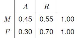
Figure 8.6: Row proportions for the Berkeley 2 \(\times\) 2 contingency table.

The column proportions could also be calculated, but they are not meaningful if method 3 is used to collect the data. For example, the proportion of accepted applicants who are male depends on the number of male applicants and, if method 3 is used, this number is decided by Berkeley. Even if method 1 or method 2 was used it makes more sense to look at row proportions, which shows how the response (outcome) depends on the explanatory variable (sex).

It is true that \[ \hat{P}(A~|~M) > \hat{P}(A~|~F). \] However, is \(\hat{P}(A~|~M)\) so much greater than \(\hat{P}(A~|~F)\) to suggest that \(P(A~|~M) > P(A~|~F)\)? To answer this question we compare the frequencies we expect if \(P(A~|~M) = P(A~|~F)\) with the observed frequencies. What are the expected frequencies if \(P(A~|~M)=P(A~|~F)=P(A)\)?

Consider the 2691 males. The expected frequency for accepted applicants is \(P(A) \times 2691\) and for rejected applicants is \(P(R) \times 2691\). Similarly, for the 1835 females the estimated expected frequencies are \(P(A) \times 1835\) and \(P(R) \times 1835\) respectively. We do not know \(P(A)\), but we can estimate it using \[ \hat{P}(A) = \frac{1755}{4526}. \] Then, if \(P(A~|~M)=P(A~|~F)=P(A)\), the estimated expected frequency for sex=\(M\) and outcome=\(A\) is \[ \hat{P}(A) \times 2691 = \frac{1755}{4526} \times 2691 = 1043.46. \] This is exactly the same estimated expected frequency as in question 1. The estimated expected frequencies (and the residuals and standardised Pearson residuals) under the assumption that \(P(A~|~M)=P(A~|~F)\) are identical to those under the assumption that sex and outcome are independent. This makes sense: if outcome (\(Y\)) is independent of sex (\(X\)) then the probability distribution of outcome is the same for each sex. The calculations used to answer Question 1 are the same as the calculations used to answer Question 2.

8.1.3 Measures of association

If we decide that the probability of acceptance depends on sex then we should also indicate how it depends on sex and how much. How can we compare the values of 2 probabilities: \(P(A~|~M)\) and \(P(A~|~F)\)?

The difference in the probability of acceptance

\[P(A~|~M)-P(A~|~F),\] which is equal to 0 if \(P(A~|~M)=P(A~|~F)\). For the Berkeley data the estimate is \(0.445 - 0.304 \approx 0.14\).

A problem with using \(P(A~|~M)-P(A~|~F)\) is that if \(P(A~|~M)\) and \(P(A~|~F)\) are very near 0 or very near 1, the value of \(P(A~|~M)-P(A~|~F)\) will be small. For example, if

• \(P(A~|~M)=0.01\) and \(P(A~|~F)=0.001\) then \(P(A~|~M)-P(A~|~F)=0.009\);
• \(P(A~|~M)=0.41\) and \(P(A~|~F)=0.401\) then \(P(A~|~M)-P(A~|~F)=0.009\).

Although the differences are the same, the former difference seems more important since \(P(A~|~M)\) is 10 times greater than \(P(A~|F)\). The following alternatives, relative risk and odds ratio, do not have this problem.

The relative risk, a ratio of probabilities

\[\frac{P(A~|~M)}{P(A~|~F)} \qquad \left( \,\mbox{or} \qquad \frac{P(R~|~M)}{P(R~|~F)} \,\right)\] which is equal to 1 if \(P(A~|~M)=P(A~|~F)\). For the Berkeley data the relative risk of acceptance is \(\hat{P}(A~|~M)/\hat{P}(A~|~F) \approx 1.47\). The relative risk of rejection is \(\hat{P}(R~|~M)/\hat{P}(R~|~F) \approx 0.79\).

Note: we cannot infer \(\hat{P}(R~|~M)/\hat{P}(R~|~F)\) from (only) the value of \(\hat{P}(A~|~M)/\hat{P}(A~|~F)\). Therefore, it matters whether we choose to work with conditional probabilities of \(A\) or of \(R\).

The odds ratio, a ratio of odds

\[\frac{P(A~|~M)}{1-P(A~|~M)}\,\,\Bigg/\,\,\frac{P(A~|~F)}{1-P(A~|~F)},\] which is equal to 1 if \(P(A~|~M)=P(A~|~F)\). For the Berkeley data the estimate is \(\approx\) 1.84.

The odds of an event \(B\) is the ratio of the probability \(P(B)\) that the event occurs to the probability \(P(\mbox{not}B) = 1 - P(B)\) that it does not occur. If \(P(B) = \frac12\) then \(B\) and \(\mbox{not}B\) are are equally likely and so the odds of event \(B\) equals 1. If \(P(B) = \frac23\) then \(B\) has double the probability of \(\mbox{not}B\) and so the odds of event \(B\) equals 2. Some other simple cases are summarised in Figure 8.7.

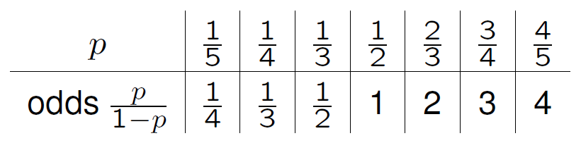
Figure 8.7: The value of the odds of an event for different probabilities \(p\) of that event.

[In the book Ross, S. (2010) A First Course in Probability, the odds ratio of an event \(B\) is defined (incorrectly in my view) as \(P(B) / (1 - P(B))\). This is a ratio of probabilities. The conventional use of the term odds ratio is for a ratio of odds.]

An odds ratio tells us how much greater the odds of an event are in one group compared to another group. The estimated odds of \(A\) for \(M\) are \(\hat{P}(A~|~M)/[1-\hat{P}(A~|~M)] \approx 0.802.\) The estimated odds of \(A\) for \(F\) are \(\hat{P}(A~|F)/[1-\hat{P}(A~|~F)] \approx 0.436.\) Therefore, the odds ratio of acceptance, comparing \(M\) to \(F\), is \(1.84 (\approx 0.802/0.436)\). The estimated odds of acceptance for males are approximately 2 times those for females. We could instead work with the conditional probabilities of the event \(R\), instead of the event \(A\). The estimated odds of \(R\) for \(M\) are \(\hat{P}(R~|~M)/[1-\hat{P}(R~|~M)] \approx 1.25 \,\,\,(=1/0.802).\) The estimated odds of \(R\) for \(F\) are \(\hat{P}(R~|F)/[1-\hat{P}(R~|~F)] \approx 2.29 \,\,\,(=1/0.436).\) When we change from considering \(A\) to \(R\), the effect is to take the reciprocal of the odds. That is,

\[ \frac{P(R \mid M)}{1 - P(R \mid M)} = \left[\frac{P(A \mid M)}{1 - P(A \mid M)}\right]^{-1} \quad \mbox{and} \quad \frac{P(R \mid F)}{1 - P(R \mid F)} = \left[\frac{P(A \mid F)}{1 - P(A \mid F)}\right]^{-1}. \] Therefore, the estimated odds of \(R\), comparing males to females, is the reciprocal of the odds of \(A\) comparing males to females. Since \(1/1.84 \approx 1/2\), we could say that the estimated odds of rejection for males are approximately a half of those for females.

The main point is that, when estimating the odds ratio, it doesn’t matter whether we work with \(P(A~|~M)\) and \(P(A~|~F)\) or \(P(R~|~M)\) and \(P(R~|~F)\), provided that we remember when we interpret the estimate of the odds.

Odds ratio and relative risk

There are two more reasons to prefer the odds ratio.

• The value of the odds ratio does not change if we treat sex as the response variable instead of outcome. This is not true of the relative risk. It can be shown, using Bayes’ theorem, that \[ \displaystyle\frac{\displaystyle\frac{P(A~|~M)}{1-P(A~|~M)}}{\displaystyle\frac{P(A~|~F)}{1-P(A~|~F)}} \,\,\,=\,\,\, \frac{\displaystyle\frac{P(M~|~A)}{1-P(M~|~A)}}{\displaystyle\frac{P(M~|~R)}{1-P(M~|~R)}}, \] that is, the odds ratio of acceptance, comparing males to females, is equal to the odds ratio of being male, comparing acceptance to rejection. With odds ratios it doesn’t matter which variable we treat as the response

• For some datasets it is not possible to estimate the relative risk. Consider the 2-way contingency table in Figure 8.8.

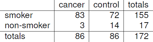
Figure 8.8: Example data from a case-control study. Source: Dorn, H.F. (1954) The relationship of cancer of the lung and the use of tobacco. American Statistician, 8, 7–13.

These data comes from a very old case-control study, designed to investigate the link between smoking and lung cancer. The idea is to compare the smoking habits of people with lung cancer (the cases) and people without lung cancer, but who are otherwise similar to the cases (the controls). The people conducting the study decided to have equal number of cases and controls: 86 of each. That is, they fixed both column totals at 86. Therefore, this is not a random sample of people from the population: if we did sample people randomly from the population then we would expect to obtain far fewer people with lung cancer than people without lung cancer. Each person was asked whether they were a smoker or non-smoker.

Let \(L\) be the event that a person has lung cancer and let \(S\) the event that a person is a smoker. We can estimate \(P(S \mid L)\) and \(P(S \mid \mbox{not}L)\): \(\hat{P}(S \mid L) = 83/86 \approx 0.97\) and \(\hat{P}(S \mid \mbox{not}L) = 72/86 \approx 0.84\). If we condition on \(L\) or on \(\mbox{not}L\) then we can treat smoking status as being randomly-sampled from the populations of people with and without lung cancer, because the row totals were not fixed. Both these estimates are high, because smoking was more prevalent in the 1950s, and \(\hat{P}(S \mid L) > \hat{P}(S \mid \mbox{not}L)\), that is, smoking is more prevalent among people with lung cancer than those who do not have lung cancer. We can estimate the odds ratio of smoking, comparing smokers to non-smokers, using \[ \displaystyle\frac{\displaystyle\frac{\hat{P}(S \mid L)}{1-\hat{P}(S \mid L)}}{\displaystyle\frac{\hat{P}(S \mid \mbox{not}L)}{1-\hat{P}(S \mid \mbox{not}L)}} = \displaystyle\frac{\displaystyle\frac{83/86}{3/86}}{\displaystyle\frac{72/86}{14/86}} = \frac{83 \times 14}{72 \times 3} = 5.38. \]

Can we estimate the relative risk? No we cannot. In this example, the relative risk of interest is \(P(L \mid S) / P(L \mid \mbox{not}S)\): we compare the probabilities of developing lung cancer for smokers and non-smokers. However, the way that these data have been sampled means that they provide no information about \(P(L)\), that is, the proportion of people in the population who have lung cancer. The proportion of people in the sample who have lung cancer has been fixed at \(1/2\) by the people who designed the study, because they fixed the column totals. Similarly, we cannot use these data to estimate \(P(L \mid S)\) or \(P(L \mid \mbox{not}S)\), the proportion of people with lung cancer will also be artificially high within the smoker and for non-smoker categories.

However, can estimate the odds ratio that we would like, that is, the odds ratio of lung cancer, comparing smoker to non-smokers, because this is equal to the estimate of 5.38 that we calculated above, owing to

\[ \displaystyle\frac{\displaystyle\frac{P(L \mid S)}{1-P(L \mid S)}}{\displaystyle\frac{P(L \mid \mbox{not}S)}{1-P(L \mid \mbox{not}S)}} \,\,\,=\,\,\, \frac{\displaystyle\frac{P(S \mid L)}{1-P(S \mid L)}}{\displaystyle\frac{P(S \mid \mbox{not}L)}{1-P(S \mid \mbox{not}L)}}. \]

Finally, we note that in cases where the events of interest happen very rarely, that is, they have very small probabilities, then the relative risk and the odds ratio have similar values. This is because when a probability \(p\) is close to \(0\), \(p/(1-p) \approx p\). Therefore, in studies of a rare disease an estimated odds ratio is often taken as an estimate of a relative risk.

8.2 3-way contingency tables

Figure 8.9 shows the 2 \(\times\) 2 \(\times\) 6 contingency table that results from classifying applicants according to 3 categorical variables: sex (\(X\)), outcome (\(Y\)) and department (\(Z\)). We now have a 2-way contingency table, like the one we analysed in Section 8.1, in each of the 6 departments.

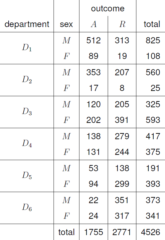
Figure 8.9: 3-way contingency table for the Berkeley admissions data.

In a 3-way contingency table there are many possible associations that we could examine. We consider the following cases.

Mutual independence. We consider 3 variables at once, that is, outcome, sex and department.

Marginal independence. We consider 2 variables, ignoring the value of the third variable, that is, outcome and sex (we have already done this), outcome and department, sex and department;

Conditional independence. We consider 2 variables separately for each value of the third variable, e.g. outcome and sex separately with each department.

8.2.1 Mutual independence

We examine whether the categorical random variables sex, outcome and department are mutually independent, that is, there are no relationships between these three variables. We have already seen in Section 8.1 that the data suggest that outcome and sex are not independent. If outcome and sex are not independent then outcome, sex and department cannot be mutually independent.

We consider how to estimate expected frequencies under the assumption that outcome, sex and department are mutually independent. (We will not actually calculate them though.) The approach we use is the same one we used for the 2-way table: we estimate the expected frequencies under the assumption that these variables are mutually independent.

How can we estimate these expected frequencies?

We take sex=\(M\), outcome=\(A\) and department=\(D_1\) as an example. If sex, outcome and department are mutually independent then \[ P(M, A, D_1) = P(M)\,P(A)\,P(D_1). \] We do not know \(P(M), P(A)\) or \(P(D_1)\), so we estimate them using the proportions in the observed data: \[ \hat{P}(M)=\frac{2691}{4526}, \quad \hat{P}(A)=\frac{1755}{4526}, \quad \hat{P}(D_1)=\frac{933}{4526}. \] Therefore, the expected frequency for sex=\(M\), outcome=\(A\) and department=\(D_1\) is estimated by \[ \frac{2691}{4526} \times \frac{1755}{4526} \times \frac{933}{4526} \times 4526 = \frac{2691 \times 1755 \times 933}{4526^2} = 215.1. \] The other expected frequencies are estimated similarly. Extending our previous notation in an obvious way we have \[ \hat{\mu}_{ijk} = n\,\hat{p}_{i++}\,\hat{p}_{+j+}\,\hat{p}_{++k} = \frac{n_{i++}\,n_{+j+}\,n_{++k}}{n^2}, \] where \[ \hat{p}_{i++} = \frac{n_{i++}}{n}, \qquad \hat{p}_{+j+} = \frac{n_{+j+}}{n}, \qquad \hat{p}_{++k} = \frac{n_{++k}}{n}. \]

8.2.2 Marginal independence

We produce marginal 2-way contingency tables by ignoring one of the variables, and examine the association between the remaining 2 variables. We have already looked at the association between outcome and sex.

Firstly we look at the association between sex and department. This gives a 2 \(\times\) 6 contingency table. The observed and estimated expected frequencies and the standardised Pearson residuals are given in Figures 8.10 and 8.11.

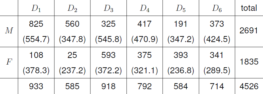
Figure 8.10: Observed and estimated expected values for sex and department.

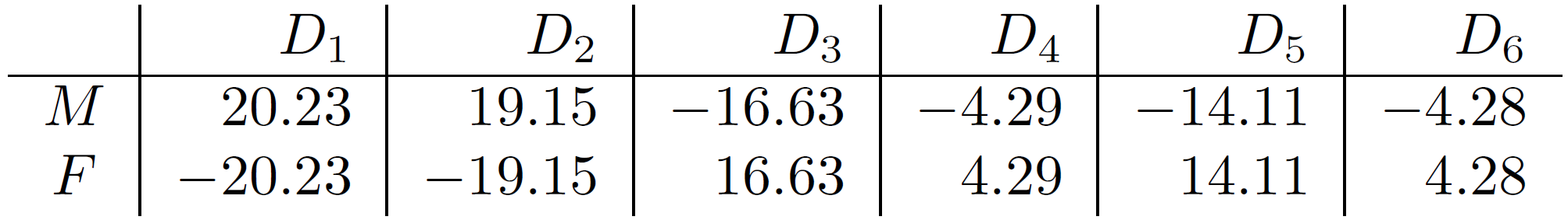
Figure 8.11: Standardised Pearson residuals for sex and department.

Note: the

• estimated expected frequencies preserve the row and column totals;
• residuals sum to zero across rows and down columns.
• standardised Pearson residuals sum to zero down columns.

We can see that many more males apply to departments 1 and 2, and many more females apply to departments 3 and 5 than we could expect if sex and department are independent. We can also see this from the estimated conditional probabilities in Figure 8.12.

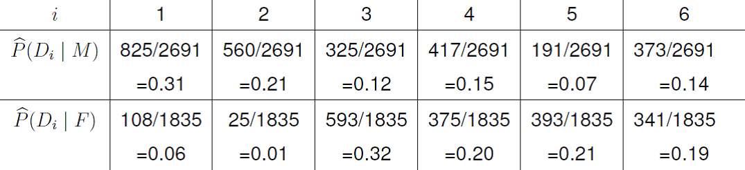
Figure 8.12: Estimated conditional probabilities of department given sex.

There does appear to be an association between sex and department. It seems that males prefer to apply to department 1 and 2 while females prefer to apply to departments 3 and 5.

Is there association between department and outcome? It turns out that department and outcome do appear to be associated. In particular the probability of acceptance in departments 1 and 2 seem to be much greater than the probability of acceptance in department 3 and 5, as we can see from the estimates in Figure 8.13.

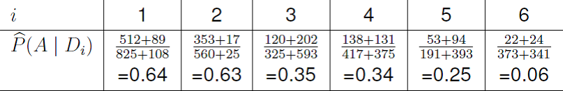
Figure 8.13: Estimated conditional probabilities of acceptance given department.

8.2.3 Conditional independence

Now we look at the association between sex and outcome separately within each department. We simply analyse each of the six 2 \(\times\) 2 tables in Figure 8.9. In other words we condition on the value of department, for example, department=1, ignoring the data from other departments. Then we examine whether sex and outcome are conditionally independent given that department=1. We do this for each department in turn.

Since it is likely that decisions to accept or reject a candidate are taken within each department, it makes sense to ask whether there is any sexual discrimination within each department. Figure 8.14 summarises the observed frequencies and estimated expected frequencies under the assumption that outcome is independent of sex and the standardised Pearson residuals.

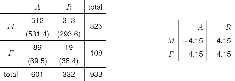
Figure 8.14: Left: 2 \(\times\) 2 contingency table for department 1. Right: standardised residuals.

The size of the standardised Pearson residual suggests that outcome and sex are not independent. In fact more females are accepted to department 1 than would be expected if outcome and sex are independent. We can also see this from the estimated conditional probabilities in Figure 8.15.

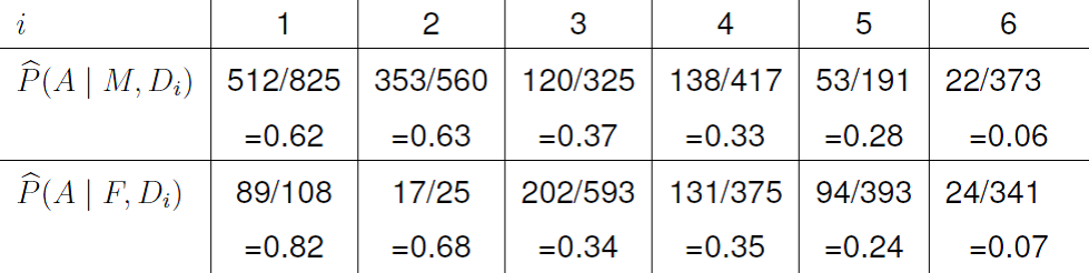
Figure 8.15: Estimated conditional probabilities of acceptance given sex and department.

We leave the calculation of estimated expected frequencies and residuals for departments 2 to 6 as an exercise. The Figure 8.16 gives the standardised Pearson residuals for the \((M, A)\) cell.

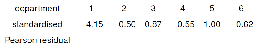
Figure 8.16: Standardised Pearson residuals for the \((M, A)\) cell by department.

A positive value indicates that more males were accepted than would be expected if outcome and sex are independent, whereas a negative value indicates that more females were accepted than would be expected. In only one department, department 1, do the data seem inconsistent with outcome and sex being independent. In this department females seem to have a higher probability of acceptance. Note, this may not be a result of discrimination in favour of females: there may be other data that explain why this happens.

8.2.4 Confounding variables

We have observed the following.

• Analysis of the 2-way table of outcome and sex suggests that the probability of acceptance is greater for males than for females.
• Analysis of the six 2-way tables of outcome and sex within each department suggests that in departments 2 to 6 outcome and sex are independent, and in department 1 females have a higher probability of acceptance.

In other words, the association between outcome and sex is different in the marginal 2 \(\times\) 2 table than in the six conditional 2 \(\times\) 2 tables.

Is there an explanation for this? The data suggest that

• department is dependent on sex: females tend to apply to different departments to males;
• outcome is dependent on department: some departments have lower acceptances rates than others.

The apparent association between sex and outcome seems actually to be a combined effect of (a) sex affecting department, and (b) department affecting outcome. Sex does not seem to affect outcome directly. Females are more likely than males to apply to the departments into which it is more difficult to be accepted.

The estimated association between sex and outcome depends on the value of the variable department. It is not uncommon for the estimated association between two variables to change depending on the value of a third variable, a so-called confounding or lurking variable. To confound means to confuse, surprise or mix up. To lurk means to hide in the background, perhaps with sinister intent! In this example, department is the confounding variable. Simpson’s paradox describes extreme cases of this, where the direction or nature of the estimated association changes or perhaps disappears. Misleading inferences could be produced if we are not aware of the effects of the confounding variable.

The moral is that it can be dangerous to ‘collapse’ a 3-way contingency table down to a 2-way contingency table, by ignoring a variable. If we move from a 3-way table to a 2-way table without analysing the 3-way table we may be throwing away important data.