Chapter 9 Linear regression

In this chapter, and Chapter 10, we examine the relationship between 2 continuous variables. First we consider regression problems, where the distribution of a response variable \(Y\) is thought to be dependent on the value of an explanatory variable \(X\). Possible aims are (a) to understand the relationship between \(Y\) and \(X\), or (b) to predict \(Y\) from the value of \(X\). We examine the conditional distribution of the random variable \(Y\) given that \(X=x\), that is, \(Y \mid X=x\). In particular, we study a simple linear regression model in which the conditional mean \(\mbox{E}(Y \mid X=x)\) of \(Y\) given that \(X=x\) is assumed to be a linear function of \(x\) and the conditional variance \(\mbox{var}(Y \mid X=x)\) of \(Y\) is assumed to be constant. That is, \[ \mbox{E}(Y \mid X=x) = \alpha+\beta\,x \qquad \mbox{and} \qquad \mbox{var}(Y \mid X=x)=\sigma^2, \] for some constants \(\alpha, \beta\) and \(\sigma^2\).

In many cases it is clear which variable should be the response variable \(Y\) and which should be the explanatory variable \(X\). For example,

• If changes in \(x\) cause changes in \(Y\), so that the direction of dependence is clear. For example, \(x\)=river depth influencing \(Y\)=flow rate.
• If the values of \(X\) are controlled by an experimenter and then the value of \(Y\) is observed. For example, \(x\)=dosage of drug and \(Y\)=reduction in blood pressure. This is sometimes called regression sampling.
• If we wish to predict \(Y\) using \(x\). For example, \(x\)=share value today and \(Y\)=share value tomorrow.

In a related, but different, problem the 2 random variables \(Y\) and \(X\) are treated symmetrically. The question is how these random variables are associated. A measure of strength of linear association between 2 variables is given by a correlation coefficient (see Chapter 10).

Regression answers the question “How does the conditional distribution of the random variable \(Y\) depend on the value \(x\) of \(X\)?”. Correlation answers the question “How strong is any linear association between the random variables \(Y\) and \(X\)?”. In a regression problem we assume that the \(Y\) values are random variables (that is, subject to random variability) but the \(x\) values are not. When using a correlation coefficient we assume that both \(X\) and \(Y\) are random variables.

9.1 Simple linear regression

We use a small set of data, and some physical theory, to estimate the age of the Universe! In 1929 the famous astronomer Edwin Hubble published a paper (Hubble (1929)) reporting a relationship he had observed (using a telescope) between the distance of a nebula (a star) from the Earth and the velocity (the recession velocity) with which it was moving away from the Earth. Hubble’s data are given in Table 9.1. A scatter plot of distance against velocity is given in Figure 9.2.

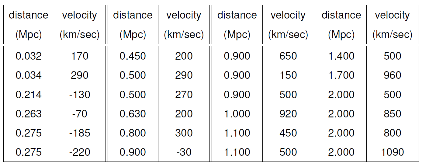
Figure 9.1: Hubble’s data. 1 MPc = 1 megaparsec = \(3.086 \times 10^{19}\) km. A megaparsec is a long distance: the distance from the Earth to the Sun is ‘only’ \(1.5 \times 10^8\) km.

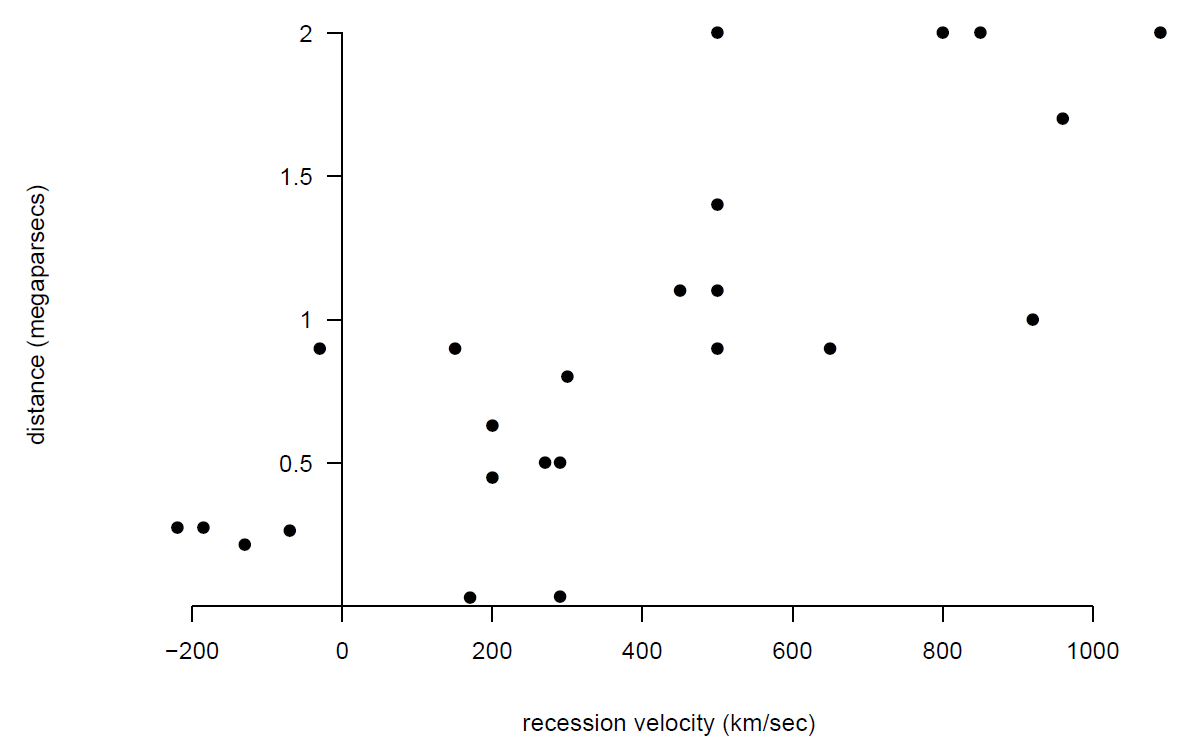
Figure 9.2: Scatter plot of distance against recession velocity.

It appears that distance and velocity are positively associated: the values of distance tend to be larger for nebulae with large velocities than for nebulae with smaller velocities. Also, this relationship appears to be approximately linear, at least over the range of velocities available.

Scientists then wondered how the positive linear association between distance and velocity could have arisen. The result was ‘Big Bang’ theory. This theory proposes that the Universe started with a Big Bang at a single point in space a very long time ago, scattering material around the surface of an ever-expanding sphere. If Big Bang theory is correct then the relationship between distance (\(Y\)) and recession velocity (\(X\)) should be of the form \[ Y = T X, \] where \(T\) is the age of the Universe when the observations were made. This is called Hubble’s Law. In other words, distance, \(Y\), should depend linearly on velocity, \(X\). \(H=1/T\) is called Hubble’s constant.

The points in Figure 9.2 do not lie exactly on a straight line, partly because the values of distance are not exact: they include measurement error. Also, there may have been astronomical events since the Big Bang which have weakened further the supposed linear relationships between distance and velocity. If we look at nebulae with the same value, \(x\), of velocity the measured value of distance, \(Y\), varies from one nebulae to another. For example, the 4 nebulae with velocities of 500 km/sec have have distances 0.9, 1.1, 1.4 and 2.0 MPc. So, for a given value of velocity there is variability in their distances from the Earth. Therefore, \(Y \mid X=x\) is a random variable, with conditional mean \(\mbox{E}(Y \mid X=x)\) and conditional variance \(\mbox{var}(Y \mid X=x)\).

In Figure 9.2 it looks possible that there is a straight line relationship between \(\mbox{E}(Y \mid X=x)\) and \(x\). Therefore we consider fitting a simple linear regression model of \(Y\) on \(x\). You could think of this as a way to draw a ‘line of best fit’ through the points in Figure 9.2.

9.1.1 Simple linear regression model

We assume that \[\begin{equation} Y_i = \alpha + \beta\,x_i + \epsilon_i, \qquad i=1,\ldots,n, \tag{9.1} \end{equation}\] where \(\epsilon_i, i=1, \ldots, n\) are error terms, representing random ‘noise’. The \(\alpha + \beta\,x_i\) part of the model is the systematic part. The \(\epsilon_i\) is the random part of the model. It is assumed that, for \(i = 1, ..., n\), \[ \mbox{E}( \epsilon_i)=0, \qquad \mbox{and} \qquad \mbox{var}( \epsilon_i)=\sigma^2, \] and that \(\epsilon_1, \ldots, \epsilon_n\) are uncorrelated. We will study correlation in the next section. It is a measure of the degree of linear association between two random variables. Uncorrelated random variables have no linear association. \(\epsilon_1, \ldots, \epsilon_n\) are uncorrelated if each pair of these variables is uncorrelated.

Another way to write down this model is, for \(i=1,\ldots,n\), \[ \mbox{E}(Y_i \mid X=x_i) = \alpha+\beta\,x_i, \qquad\quad (\mbox{straight line relationship}), \] and \[ \qquad \mbox{var}(Y_i \mid X=x_i)=\sigma^2, \qquad\quad (\mbox{constant variance}), \] where, given the values \(x_1,\ldots,x_n\), the random variables \(Y_1, \ldots, Y_n\) are uncorrelated.

Figure 9.3 shows how the conditional distribution of \(Y\) is assumed to vary with the value of \(x\).

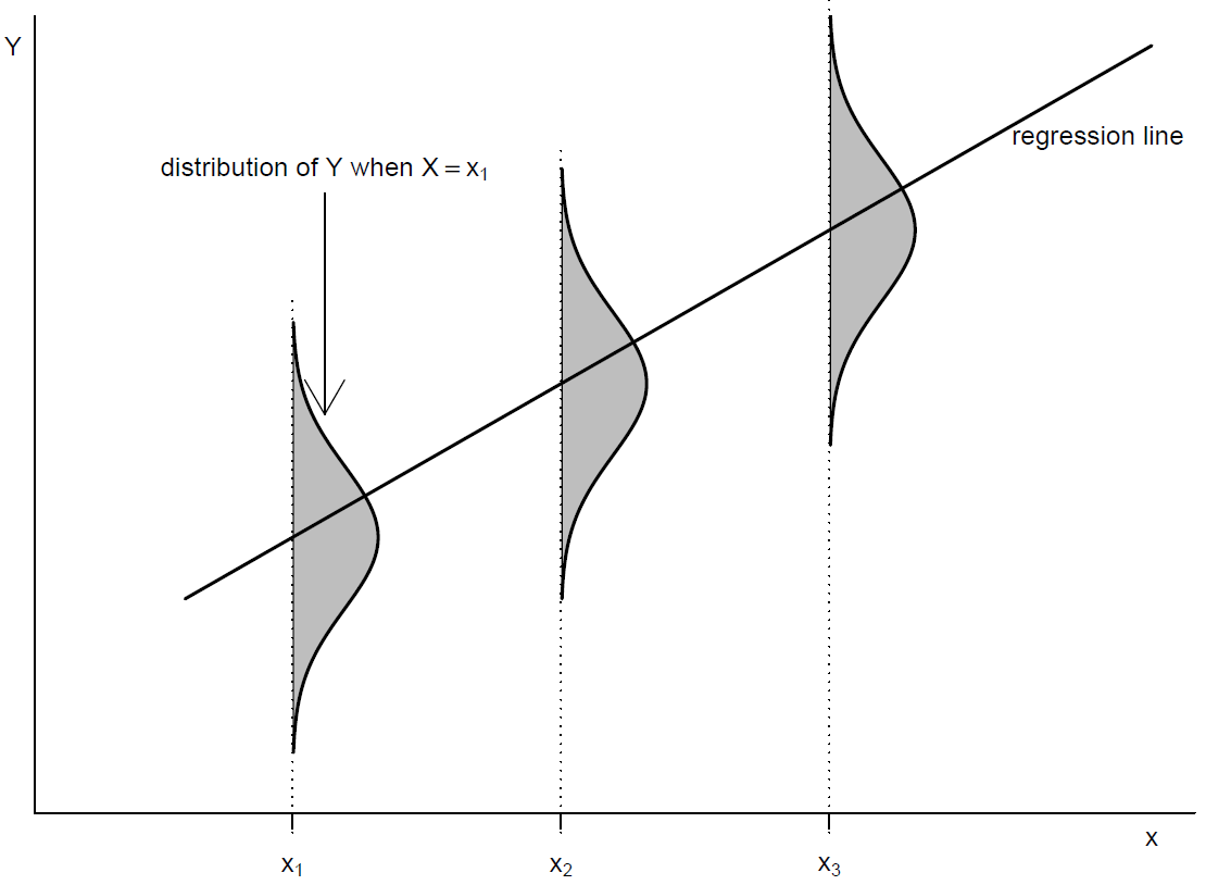
Figure 9.3: Conditional distribution of \(Y\) given \(X=x\) for a linear regression model.

Interpretation of parameters

• Intercept: \(\alpha\). The expected value (mean) of \(Y\) when \(X=0\), that is, \(\mbox{E}(Y~|~X=0)\).
• Gradient or slope: \(\beta\). The amount by which the mean of \(Y\) given \(X=x\), \(\mbox{E}(Y~|~X=x)\), increases when \(x\) is increased by 1 unit. That is, \[ \beta = \mbox{E}(Y~|~X=x+1)- \mbox{E}(Y~|~X=x). \]
• Error variance: \(\sigma^2\). The variability of the response about the linear regression line (in the vertical direction).

9.1.2 Least squares estimation of \(\alpha\) and \(\beta\)

Suppose that we have paired data \((x_1,y_1), \ldots, (x_n,y_n)\). How can we fit a simple linear regression model to these data? Initially, our aim is to use estimators \(\hat{\alpha}\) and \(\hat{\beta}\) of \(\alpha\) and \(\beta\) to produce an estimated regression line \[ y= \hat{\alpha}+\hat{\beta}\,x. \] There are many possible estimators of \(\alpha\) and \(\beta\) that could be used. A standard approach, which produces estimators with some nice properties is least squares estimation. Firstly, we rearrange equation (9.1) to define residuals \[ R_i = Y_i-(\hat{\alpha}+\hat{\beta}\,x_i) = Y_i-\hat{Y}_i, \qquad i=1,\ldots,n, \] the differences between the observed values \(Y_i, i = 1, \ldots, n\) and the fitted values \(\hat{Y}_i=\hat{\alpha}+\hat{\beta}\,x_i\), \(i = 1, \ldots, n\) given by the estimated regression line.

The least squares estimators have the property that they minimise the sum of squared residuals: \[ \sum_{i=1}^n \left(Y_i-\hat{\alpha}-\hat{\beta}\,x_i\right)^2. \]

It is possible to do this by hand to give \[\begin{equation} \hat{\beta}=\frac{\displaystyle\sum_{i=1}^n \left(x_i- \overline{x}\right)\,\left(Y_i- \overline{Y}\right)} {\displaystyle\sum_{i=1}^n \left(x_i- \overline{x}\right)^2} = \frac{C_{xY}}{C_{xx}} \qquad \mbox{and} \qquad \hat{\alpha}= \overline{Y} - \hat{\beta}\, \overline{x}, \end{equation}\] where \(\overline{Y} = (1/n)\sum_{i=1}^n Y_i\) and \(\overline{x} = (1/n)\sum_{i=1}^n x_i\). Note: \(\hat{\alpha}\) and \(\hat{\beta}\) are each linear combinations of\(Y_1,\ldots,Y_n\).

For a given set of data the minimised sum of squared residuals is called the residual sum of squares (RSS), that is, \[ RSS = \sum_{i=1}^n \left(Y_i-\hat{\alpha}-\hat{\beta}\,x_i\right)^2 = \sum_{i=1}^n r_i^{\,\,2} = \sum_{i=1}^n \left(Y_i-\hat{Y}_i\right)^2. \]

Estimating \(\sigma^2\). There is one remaining parameter to estimate; the error variance \(\sigma^2\). The usual estimator is \[\begin{equation} \hat{\sigma}^2 = \frac{RSS}{n-2}. \end{equation}\] An estimate of \(\sigma^2\) is important because it quantifies how much variability there is about the assumed straight line relationship between \(Y\) and \(x\).

Properties of estimators. It can be shown that \[ \mbox{E}(\hat{\alpha})=\alpha, \quad \mbox{E}(\hat{\beta})=\beta, \quad \mbox{E}(\hat{\sigma}^2)=\sigma^2, \] that is, these estimators are unbiased for the parameters they are intended to estimate. It can also be shown that the least squares estimators \(\hat{\alpha}\) and \(\hat{\beta}\) have the smallest possible variances of all unbiased estimators of \(\alpha\) and \(\beta\) which are linear combinations of the response \(Y_1,\ldots,Y_n\).

Coefficient of determination. We may wish to quantify how much of the variability in the responses \(Y_1,\ldots,Y_n\) is explained by the values \(x_1,\ldots,x_n\) of the explanatory variable. To do this we can compare the variance of the residuals \(\{r_i\}\) with the variance of the original observations \(\{Y_i\}\), producing the coefficient of determination, \(R\)-squared, given by \[ R\text{-squared} = 1- \frac{RSS}{\displaystyle\sum_{i=1}^n \left(Y_i-\bar{Y}\right)^2} = 1-\frac{\mbox{variability in $Y$ not explained by $x$}} {\mbox{total variability of $Y$ about $\bar{Y}$}}, \] where \(0 \leq R\text{-squared} \leq 1\). Think of \(R\text{-squared}\) as a name, not literally as the square of a quantity \(R\). \(R\text{-squared}=1\) indicates a perfect fit; \(R\text{-squared}=0\) indicates that none of the variability in \(Y_1,\ldots,Y_n\) is explained by \(x_1,\ldots,x_n\), producing a horizontal regression line (\(\hat{\beta}=0\)). The value of \(R\text{-squared}\), perhaps expressed as a percentage, is often quoted when a simple linear regression model is fitted. This gives an estimate of the percentage of variability in \(Y\) that is explained by \(x\).

9.1.3 Least squares fitting to Hubble’s data

Figures 9.4, 9.5 and 9.6 show least squares regression lines under 3 different models:

• Model 1. \(Y\) does not depend on \(X\), so that

\[ Y_i = \alpha_1 + \epsilon_i, \qquad i=1,\ldots, n. \]

• Model 2. \(Y\) depends on \(X\) according to Hubble’s law, so that

\[ Y_i = \beta_2\,x_i + \epsilon_i, \qquad i=1,\ldots, n, \]

where \(\beta_2=T\) is the age of the Universe.

• Model 3. \(Y\) depends on \(X\) according to the full linear regression model

\[ Y_i = \alpha_3+\beta_3\,x_i + \epsilon_i, \qquad i=1,\ldots, n. \]

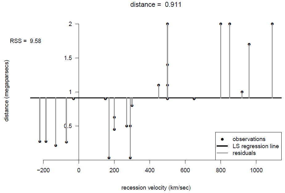
Figure 9.4: Scatter plot of distance against recession velocity, with least squares fit of a horizontal line.

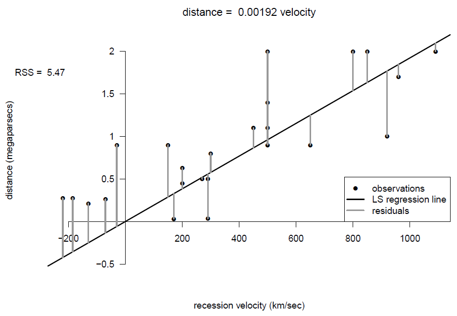
Figure 9.5: Scatter plot of distance against recession velocity, with least squares fit of a line through the origin.

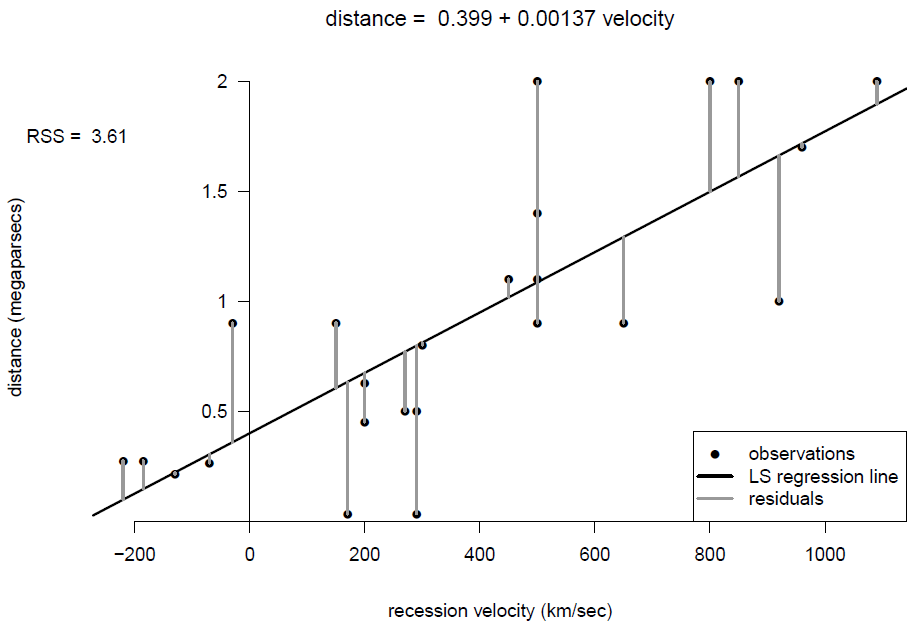
Figure 9.6: Scatter plot of distance against recession velocity, with least squares fit of an unconstrained line.

These figures also shows the sizes of the residuals and the residual sums of squares \(RSS\). From the plots, and the relative sizes of \(RSS\), it seems clear that velocity \(x\) explains some of the variability in the values of distance \(Y\). The residual sum of squares, \(RSS_3\), of Model 3 is smaller than the residual sum of squares, \(RSS_2\), of Model 2. It is impossible that \(RSS_3 > RSS_2\).

A key question is whether \(RSS_3\) is so much smaller than \(RSS_2\) that we would choose Model 3 over Model 2, which is a question that is considered in STAT0003. Model 2 is an example of regression through the origin, where it is assumed that the intercept equals 0. We should only fit this kind of model if we have a good reason to. Here Hubble’s Law gives us a good reason. Note that for a regression through the origin, we use \(\hat{\sigma}^2 = RSS/(n-1)\).

Since we want to estimate the age of the Universe, we use the estimated regression line for Model 2: \[ y = 0.00192\,x. \] Therefore, the estimated age of the Universe is given by \[ \hat{T}=0.00192 \mbox{ Mpc/km/sec}. \] To clarify the units of \(\hat{T}\) we need to convert MPcs to kms by multiplying by \(3.086 \times 10^{19}\). This gives \(\hat{T}\) in seconds. We convert to years by dividing by \(60 \times 60 \times 24 \times 365.25\): \[ \hat{T} = 0.00192 \times \frac{3.086 \times 10^{19}}{60 \times 60 \times 24 \times 365.25} \approx 2 \mbox{ billion years}. \]

Update

Since Hubble’s work, physicists have obtained more data in order to obtain better estimates of distances of nebulae from the Earth and hence the age of the Universe. Figure 9.7 shows an example of these data (Freedman et al. (2001)). Using more powerful telescopes, it has been possible to estimate the distances of nebulae which are further from the Earth. Having a wider range of distances gives a better (smaller variance) estimator of the age of the Universe.

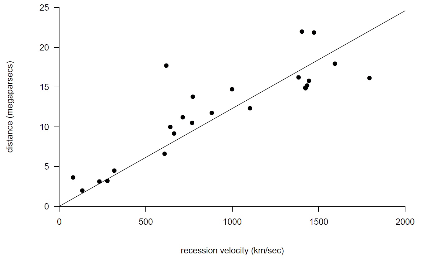
Figure 9.7: Scatter plots of new ‘Hubble’ data with fitted regression through the origin.

Using these data we obtain \(\hat{T}=0.0123\) which gives \[ \hat{T} = 0.0123 \times \frac{3.086 \times 10^{19}}{60 \times 60 \times 24 \times 365.25} \approx 12 \mbox{ billion years}. \] This estimate agrees more closely with current scientific understanding of the age of the Universe than Hubble original estimate.

9.1.4 Normal linear regression model

It is common to make the extra assumption that the errors are normally distributed: \[ \epsilon_i \sim N(0,\sigma^2), \qquad i=1,\ldots,n. \] In other words \[ Y_i \mid X=x_i \sim N(\alpha+\beta\,x_i,\sigma^2), \qquad i=1,\ldots,n. \] This assumption can be used to (a) decide whether the explanatory variable \(x\) is needed in the model, and (b) produce interval estimates of \(\alpha, \beta, \sigma^2\) and for predictions made from the model. These tasks are beyond the scope of STAT0002, but are covered in STAT0003.

9.1.5 Summary of the assumptions of a (normal) linear regression model

1. Linearity: the conditional mean of \(Y\) given \(x\) is a linear function of \(x\).
2. Constant error variance: the variability of \(Y\) is the same for all values of \(x\).
3. Uncorrelatedness of errors: the errors are not linearly associated.
4. Normality of errors: for a given value of \(x\), \(Y\) has a normal distribution.

Uncorrelatedness and independence are related concepts.
If two random variables are independent then they are uncorrelated, that is, independence implies lack of correlation. However, the reverse is not true: two random variables can be uncorrelated but not independent (see Section 10.3.2, that is, lack of correlation does not imply independence. The only exception to this is the (multivariate) normal distribution: for example, if two (jointly) normal random variables are uncorrelated then they are independent. This explains why it is common for an alternative assumption 3. to be used:

3. Independence of errors: knowledge that one response \(Y_i\) is larger than expected based on the model does not give us information about whether a different response \(Y_j\) is larger (or smaller) than expected.

Notice that, even in the normal linear regression model, we have not made any assumption about the distribution of the \(x\)s. In some studies the values of \(x\) are chosen by an experimenter, that is, they are not random at all.

9.2 Looking at scatter plots

Before fitting a linear regression model we should look at a scatter plot of \(Y\) against \(x\) to see whether the assumptions of the linear regression model appear to be reasonable. Some questions:

1. Is the relationship between \(Y\) and \(x\) approximately linear?

2. Suppose that we imagine, or draw, a straight line (or a curve if the relationship is non-linear) through the data. Is the variability of \(Y\) (the vertical spread) of points about this straight line approximately constant for all values of \(x\)?

3. Are there any points which do not appear to fit in with the general pattern of the rest of the data?

Figure 9.8 gives some example scatter plots.

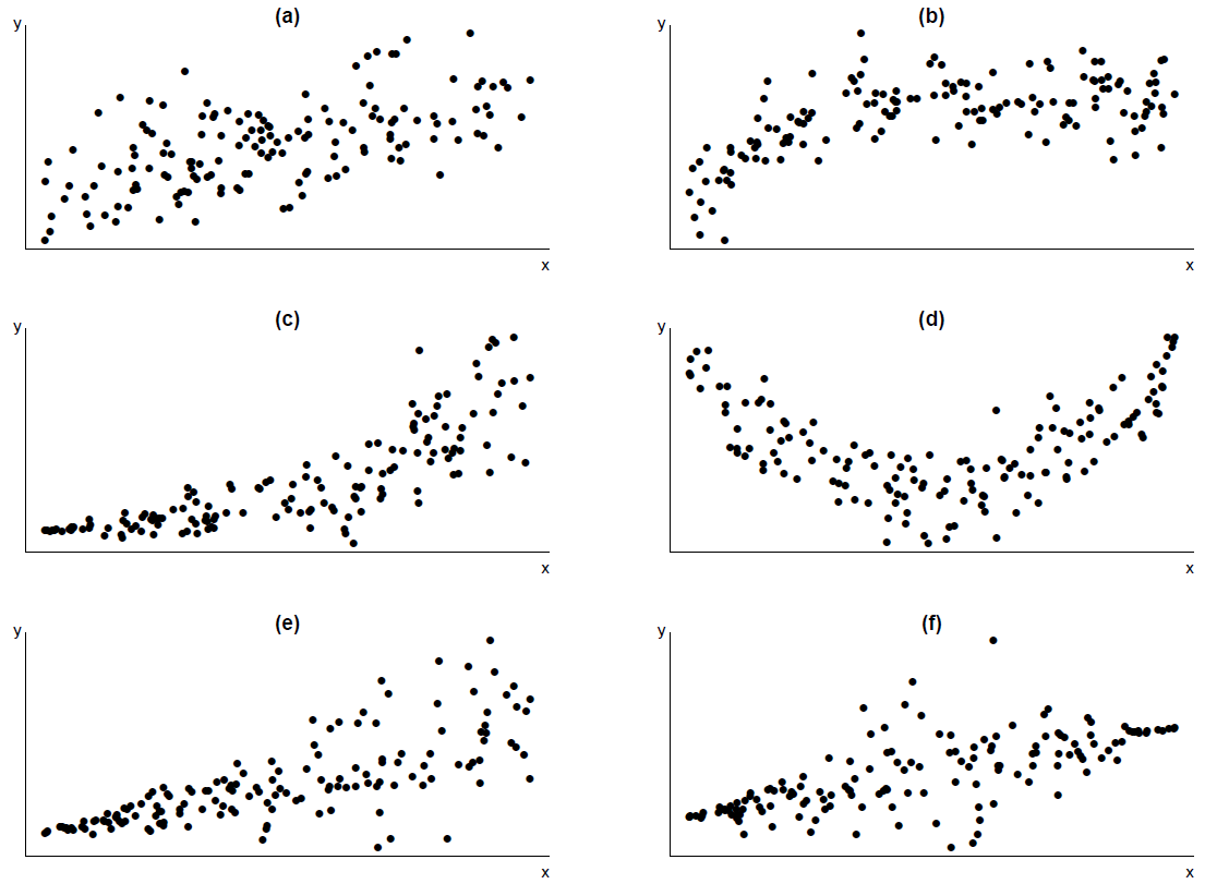
Figure 9.8: Some scatter plots.(a) (approximately) linear relationship, (approximately) constant spread about line; (b) non-linear relationship, constant spread about curve;(c) non-linear relationship, increasing spread about curve;(d) quadratic relationship, constant spread about curve; (e) linear relationship, increasing spread about line;(f) linear relationship, non-constant spread about line.

We now consider what course of action to take based on each of these plots.

1. The assumptions of linearity and constant error variance appear to be reasonable. Therefore, we fit a simple linear regression model to these data.
2. The assumption of linearity is not reasonable, but
   1. the relationship between \(Y\) and \(x\) is monotonic (increasing), and
   2. the variability in \(Y\) is approximately constant for all values of \(x\).

We could try transforming \(x\) to straighten the scatter plot, because transforming \(x\) will not affect the vertical spread of the points. The plot is like the plot in the top left of Figure 2.27, so we could try \(\log x\) or \(\sqrt{x}\). (If we transform \(Y\) then (b)(ii) would probably no longer be true.)

3. The assumption of linearity is not reasonable, but
   1. the relationship between \(Y\) and \(x\) is monotonic (increasing), and
   2. the variability in \(Y\) increases as \(x\) increases (or, equivalently, as the mean of \(Y\) increases).

We could try transforming \(Y\) to straighten the scatter plot. Transforming \(Y\) will affect the vertical spread of the points. We may be able to find a transformation of \(Y\) which both straightens the plot and makes the variability in \(Y\) approximately constant for all values of \(x\). The plot is like the plot in the bottom right of Figure 2.27, so we could try \(\log Y\) or \(\sqrt{Y}\). If not, we may need to transform both \(Y\) and \(x\). (If we transform \(x\) only then the variability of \(Y\) will still increase as \(x\) increases.)

4. The assumption of linearity is not reasonable, and
   1. the relationship between \(Y\) and \(x\) is not monotonic (it is quadratic), and
   2. the variability in \(Y\) is approximately constant for all values of \(x\).

Fit a regression model of the form \[ Y_i = \alpha+\beta_1\,x_i+\beta_2\,x_i^2 + \epsilon_i, \qquad i=1,\ldots, n. \] This is beyond the scope of STAT0002. You will study this in STAT0006.

5. The assumption of linearity is reasonable but the variability in \(Y\) increases as \(x\) increases. A transformation of \(Y\) may be able to make the variability of \(Y\) approximately constant, but it would produce a non-linear relationship. (Transforming both \(Y\) and \(x\) might work.) Even though the assumption of constant error variance is not reasonable, the least squares estimators in Section 9.1.2 are sensible (unbiased). However, it is better to use something called weighted least squares estimation (this is beyond the scope of STAT0002).

6. The assumption of linearity is reasonable but the variability in \(Y\) is small for extreme (small or large) values of \(x\) and large for middling values of \(x\). The comments made in (e) also apply here.

If we use transformation to make the assumptions of the simple linear regression model reasonable then, ideally, the transformation should make sense in terms of the subject matter of the data, and be easy to interpret. When interpreting the results of the modelling we need to take into account any transformation used. We will consider some examples where transformation is needed in Section 9.4. In the next section we consider how to check the assumptions of a model after it has been fitted.

9.3 Model checking

We consider how to use residuals to check the various assumptions of a simple linear regression model. The residual \(r_i\) is a measure of how closely a model agrees with the observation \(y_i\). Recall that we are checking for both isolated lack-of-fit (a few unusual observations) and systematic lack-of-fit (where some more general behaviour of the data is different from the model).

It is best to use graphs to examine the residuals. For many of these plots we can simply use the residuals \[ r_i = y_i-\hat{y}_i, \qquad i=1,\ldots,n. \] However, it can be helpful to standardise residuals so that they have approximately a variance of 1, if the model is true. One possibility is to divide by the estimate of \(\sigma\), that is, \(r_i/\hat{\sigma}\). However, different \(r_i\)s usually have slightly different variances. To take account of this we can use standardised residuals \[ r^S_i = \frac{r_i}{\hat{\sigma}\,\sqrt{1-h_{ii}}}, \] where \(h_{ii}\) is a number between 0 and 1 whose calculation is something that you do not need to know for STAT0002.

We consider each assumption of the model and the plot(s) which can be used to check for systematic departures from the assumption.

• Linearity. The relationship between \(\mbox{E}(Y~|~X=x)\) is linear in \(x\).

The initial plot of \(Y\) against \(x\) gives us a good idea about this. We also plot (standardised) residuals against \(x\) (or the fitted values). If the assumption of linearity is valid then we expect a random scatter of points with no obvious pattern. Patterns in the residuals may indicate a non-linear relationship between \(Y\) and \(x\).

• Constant error variance. The errors have the same variance, \(\sigma^2\).

We plot (standardised) residuals against the fitted values. If the assumption of constant variance is valid then we expect a random scatter of points with no obvious pattern. A common departure is that the variability of the residuals increases/decreases with the fitted values. This suggests that the error variance increases/decreases with \(Y\).

• Independent errors. The errors \(\{\epsilon_i\}\) should be independent.

This is an important assumption. However, it can be difficult to check, because there are many ways in which the response data could be dependent. We list some common forms of dependence below.

• Serial dependence (dependence in time). Suppose that if observation \(Y_i\) is larger (smaller) than expected under the model, giving a positive (negative) residual, then observation \(Y_{i+1}\) will tend also to be larger (smaller) than expected. In this case the successive residuals will be positively associated: the value of one residual affects the value of the next residual. In this case, if the residuals are plotted in time order, there will tend to be more groups of positive residuals and groups of negative residuals than there would be if the residuals were independent. Similarly, if the residuals are negatively associated the residuals will tend alternate from positive to negative and back again repeatedly. If the data were collected in time order (and we are given the order) we should produce a scatter plot of \(r^S_{i+1}\) against \(r^S_i\), that is, each residual against the previous residual, to check whether the size of one residual affects the size of the next residual.

• Spatial dependence. This is similar to serial dependence except that the dependence is over space rather than in time. It arises in situations where data are collected at different locations in space. It is common that observations from two nearby locations tend to be more similar to each other than observations from two distant locations. Suppose that we have time series of observations at two locations. We should produce a scatter plot of the residuals at one location against the (corresponding) residuals at the other location.

• Cluster dependence. This may occur when the data have been collected in groups. For example, suppose that we collect data on students from UCL. Two students from the same department may tend to be more similar to each other in their responses than two students from different departments. In such cases we could colour or label the points in the residual plots to reflect the department of each student, and look for patterns.

Otherwise, it is important to understand how the data were generated, and what they mean, in order to assess whether (given the values of \(x_1,\ldots x_n\)) the responses, \(Y_1,\ldots,Y_n\), can be assumed to be independent.

• Normality. If the errors \(\{\epsilon_i\}\) are assumed to have a normal distribution then the standardised residuals should have approximately a N(0,1) distribution. We can look at a histogram or a normal QQ plot of residuals.

In addition we should check these plots for any points which do not fit in with the pattern of the other residuals.

Figure 9.9 shows the plots of residuals against fitted values after fitting a linear regression model to the scatter plots in Figure 9.8. (Note that we shouldn’t really fit a linear model to the data in plots (b), (c) and (d). We do this here just to show what the residual plots look like.) You should be able to see how the residual plots relate to the original scatter plots.

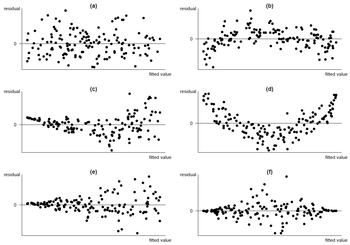
Figure 9.9: Patterns to look out for in residual plots: (a) random scatter (satisfactory); (b) non-linear, constant spread about curve; (c) non-linear, increasing spread about curve; (d) quadratic, constant spread about curve; (e) scatter about line residual=0, increasing spread about line (triangle/funnel); (f) scatter about line residual=0, non-constant spread about line (diamond).

Plot (a) is an example of a residual plot for a model that fits well: a random scatter of points about the horizontal line residual=0, with approximately constant vertical spread for all values on the \(x\)-axis. In Section 9.2 we explained, for the other plots, what the patterns in these plots implied about the relationship between the response and the explanatory variable, and we considered actions we could take in these cases.

Note that:

• We must take into account the spread of the points on the \(x\)-axes of these plots. For example, a triangular pattern can be produced just because there are more large fitted values than small fitted values (see Figure 9.10).
• The human eye is very good at picking out patterns in plot, even when these patterns do not really exist!

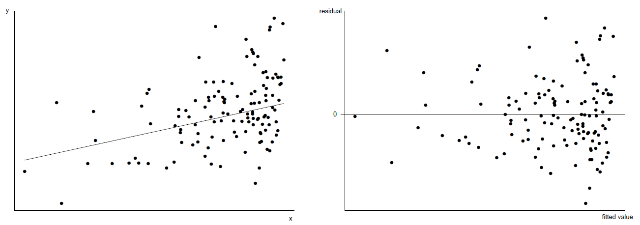
Figure 9.10: Left: scatter plot of \(y\) against \(x\). The true relationship is linear with constant error variance. Right: a triangular residual plot results from uneven distribution of \(x\) values.

Figure 9.11 shows a scatter plot where the relationship between \(\mbox{E}(Y \mid X=x)\) and \(x\) is linear and the variability in \(Y\) about this line is approximately constant. However, the distribution of \(Y\) about the line is skewed. We can see this from the scatter plot and, more clearly, in the residual plots in Figure 9.12. Although transformation of \(Y\) could make the error distribution more symmetric, it will mess up the linearity. Therefore, the action to take is to fit the linear regression model, and report the fact that the error distribution is skewed.

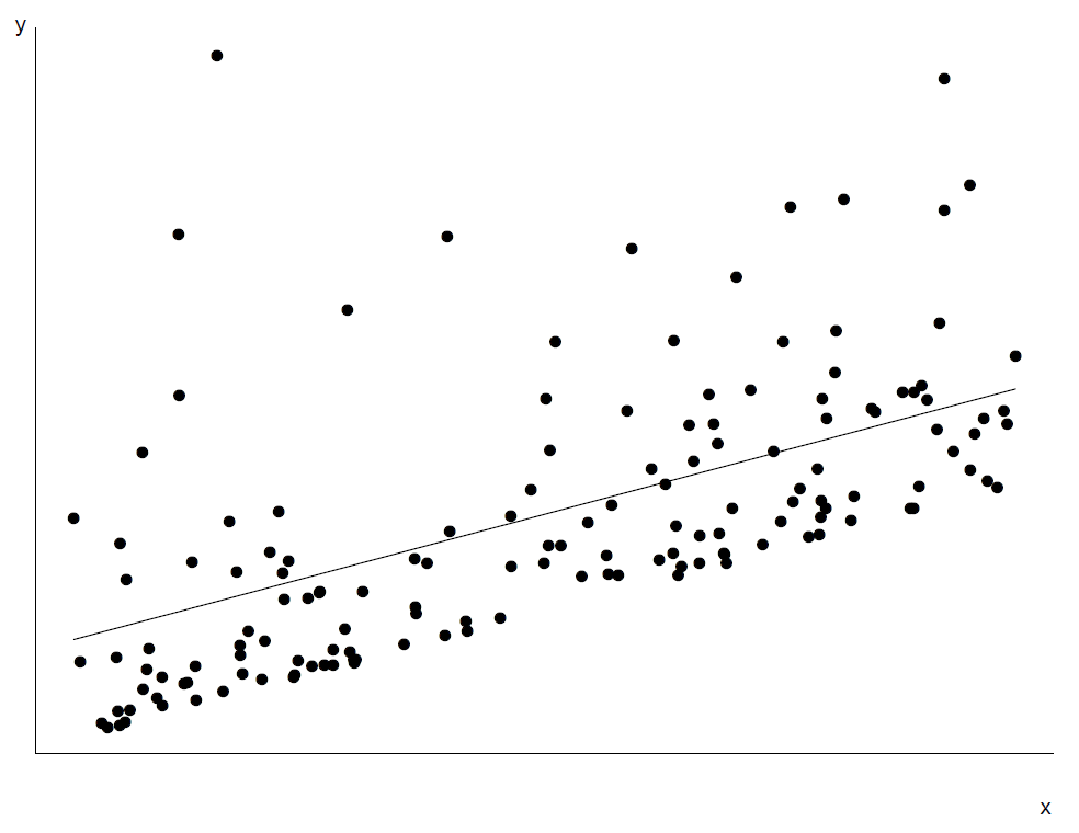
Figure 9.11: Scatter plot of \(y\) against \(x\). The true relationship is linear but the error distribution skewed (with constant variance).

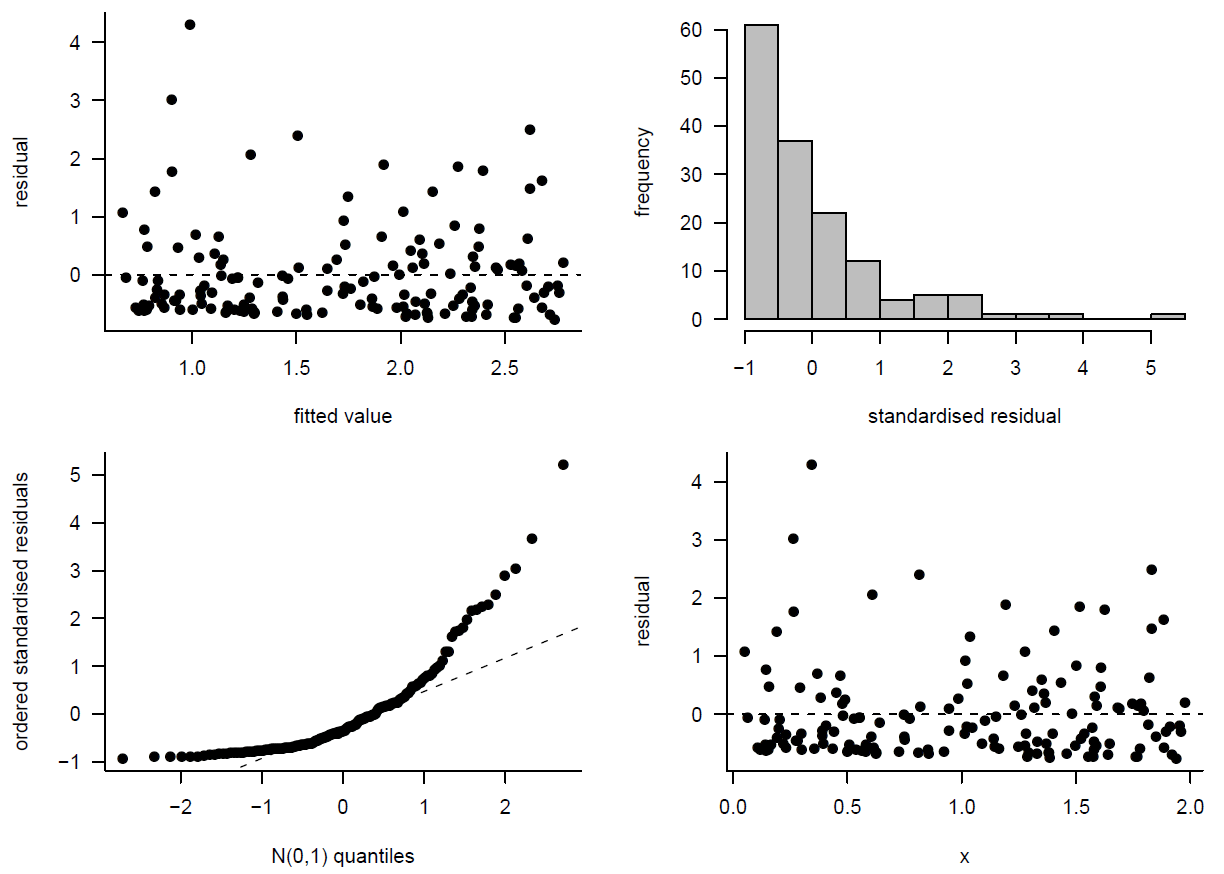
Figure 9.12: Residual plots from the linear model fitted to the data in Figure 9.11.

Transformation of \(Y\) could make the error distribution more symmetric, but it will mess up the linearity. Therefore, we fit the linear regression model, and report the fact that the error distribution is skewed.

The Hubble example (continued). We return to Hubble’s data. Figure 9.14 shows some residual plots for Model 2 and Model 3.

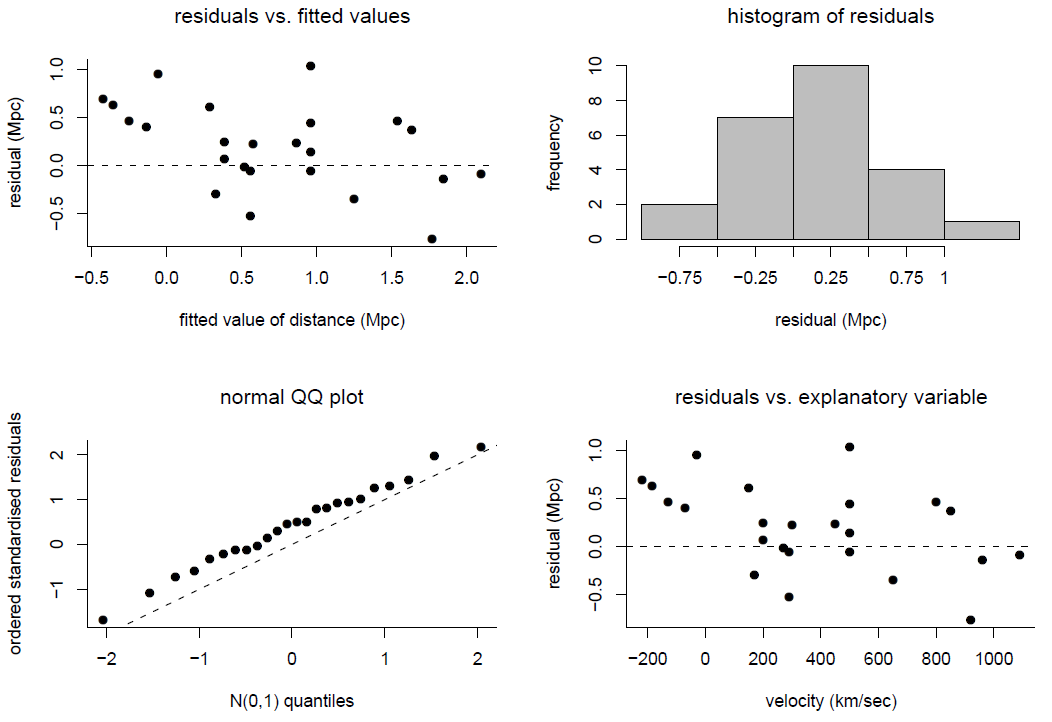
Figure 9.13: Checking the linear regression model fitted to Hubble’s data. Model 2, regression through the origin.

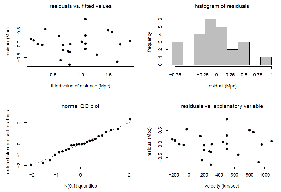
Figure 9.14: Checking the linear regression model fitted to Hubble’s data. Model 3.

There is no obvious lack-of-fit for Model 3. For Model 2 the main effect of forcing the regression line through the origin is to produce weak linear patterns in the plots of residuals against fitted values and against velocity.

9.3.1 Departures from assumptions

As we have seen in Section 9.1.5 the main assumptions underlying a (normal) linear regression model are linearity, constant error variance, independence of errors and normality of errors. Since all models are wrong (see Section 7.3 these assumptions cannot be exactly true. However, we hope that they are approximately true, or at least close enough to being true that the results from the model are useful.

• If one, or more, of these assumptions is not even approximately true, should we be worried? What should we do about it?
• Are these assumptions of equal importance? Or are particular assumptions more important than others, because even a small departure from the assumption results in our inferences being very incorrect?

We consider departures from each assumption, and what to do about them, in turn. For the moment we assume that there is a departure from only one of the assumptions.

Linearity

Departures.

1. Systematic departure. A straight line is not appropriate generally: curved relationship or two separate straight lines, e.g. one for men, one for women.
2. Isolated departure. A straight line is appropriate for most of the data but there are a small number of outliers.

Consequences.

• Bias: systematic over/under estimation and prediction of \(\mbox{E}(Y \mid X=x)\).}
• Misleading inferences: confidence intervals and standard errors (see STAT0003) do not reflect the true uncertainty, hypothesis tests of regression parameters (see STAT0003) do not have the correct properties.

Action.

1. Systematic departure. Curved relationship: transform \(Y\) and/or \(x\) to achieve approximate linearity; or fit a non-linear regression model (beyond scope of STAT0002). 2 straight lines: fit two separate regression lines, e.g. one for males and one for females.
2. Isolated departure. Check outliers (see Section 9.3.2). If outliers are kept, use a statistical method that is designed to be resistant to the presence of outliers (beyond scope of STAT0002).

Constant error variance

Departures: for example, plots (e) and (f) in Figure 9.8.

Consequences.

• The least squares estimators are still unbiased for \(\alpha\) and \(\beta\).
• Misleading inferences (as in linearity above).

Action: transform \(Y\) to achieve approximate constancy of error variance; or use weighted least squares (beyond scope of STAT0002).

Independence of errors

Departures: serial, spatial or cluster dependence.

Consequences:

• The least squares estimators are still unbiased for \(\alpha\) and \(\beta\).
• Seriously misleading inferences (as above but more affected). For example, if there is strong dependence between the errors then the amount of information in the data to estimate the model parameters is much different than if the errors are independent. Not taking this into account means that uncertainty in the estimates is misrepresented.

Action: more complicated modelling to take into account the form of the dependence (beyond scope of STAT0002).

Normality of errors

Departures: an error distribution which is not normal, for example, skewed (see Figure 9.11, light-tailed or heavy-tailed.

Consequences:

• The least squares estimators are still unbiased for \(\alpha\) and \(\beta\).
• Inferences: confidence intervals, hypothesis tests etc. are OK unless the non-normality is extreme or the sample size is small. This is because the sampling distributions of \(\hat{\alpha}\) and \(\hat{\beta}\) can be approximately normal even when the errors are not normal.
• However, prediction intervals for new observations (see STAT0003) are affected because they are based directly on the normality of the errors.

Action:

• Fit the model; report the non-normality of the error distribution.
• There may be a good reason to use a model with a different response distribution for \(Y\), for example, if the \(Y\)s are counts we could use a Poisson distribution (beyond the scope of STAT0002).

The order of importance of the assumptions for a linear model (most important first) is: linearity and independence, constant error variance, normality of errors. We may find that there are clear departures from more than one assumption, for example, the relationship between \(Y\) and \(x\) is non-linear and the error variance is not constant. If we are lucky we might find a transformation to improve both of these departures.

9.3.2 Outliers and influential observations

We have already considered the possibility of outliers. We shouldn’t remove an observation just because it appears to be an outlier. However, we should consider whether the conclusions of our analysis are not influenced strongly by outliers. An observation which influences strongly the conclusions of a statistical analysis is called an influential observation. We can assess whether an observation (or group of observations) is influential is to carry out the analysis with and without the observation, and see whether the conclusions change by a practically relevant amount. We will see that in a linear regression analysis some types of outlier are influential, whereas others are not.

Figure 9.15 shows some examples where there are one or two outlying observations. The greater the influence of the outlier(s) the greater the change in the fitted regression line when the they are removed. Generally speaking, an observation with an outlying (small or large) value of \(x\) has a greater potential (the technical term is leverage) to affect the slope of the fitted regression line than an observation which has an average \(x\) value. This can be seen by comparing plots (a) and (b).

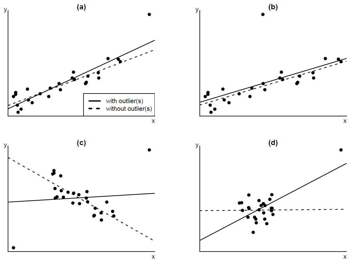
Figure 9.15: Outliers and their influence on the fitted linear regression line. The fitted line for the complete data (———) and when the outlier(s) are removed (- - - - - -) is drawn on the plots. (a) outlying \(x\) value with moderate influence on the fitted regression line; (b) average \(x\) value with small influence; (c) 2 outlying \(x\)s with large influence; (d) outlying \(x\) with large influence.

How to deal with outliers and influential observations

Before carrying out a statistical analysis the data should be checked for unusual or unexpected observations and, if possible, any errors should be corrected. Suppose that as a result of statistical analyses an observation, or group of observations, are thought to be outlying and/or influential. Then the following procedure should be followed.

1. Do the conclusions change by a practically important amount when the observation is deleted?

   1. If ``No’’: Leave the observation in the dataset;
   2. If ``Yes’’: goto 2.

2. Investigate the observation.

   1. Is the observation clearly incorrect?

      1. If ``Yes’’: if the error cannot be corrected then either use a resistant statistical method or delete the case.
      2. If ``No’’: goto 3.

   2. Is there good reason to believe that the observation does not come from the population of interest?

      1. If ``Yes’’: either use a resistant statistical method or delete the case.
      2. If ``No’’: goto 3.

3. (For linear regression.) Does the observation have an explanatory variable (\(x\)) value which is much smaller or much larger than those of the other observations?

   1. If ``Yes’’: delete the observation; refit the model; report conclusions for the reduced range of explanatory variables.
   2. If ``No’’: more data, or more information about the influential observation, are needed. Perhaps report 2 separate conclusions: one with the influential observation, one without.

There must be a good reason for deleting an observation.

9.4 Use of transformations

In Section 2.8 we found that taking a log transformation of rainfall amounts in the cloud-seeding dataset had two effects: (a) it made the values in the two groups more symmetrically distributed, and (b) made the respective sample variances more similar. In Section 9.2 we saw examples where there were clear departures from the assumptions of a linear regression model (see Section 9.1.5), but where a transformation of \(Y\) and/or \(x\) might be able to improve this.

Suppose that, either before fitting a linear regression model or afterwards (checking the model using residual plots), we find that one, or more, of the assumptions of linearity, constant variance or normality appear not to be valid.We may be able to find transformations of the response variable \(Y\) and/or the explanatory variable \(x\) for which these assumptions are more valid.However, it may not be possible to find transformations for which all the assumptions are approximately valid.

To illustrate this we return to the 2000 US Presidential Election example. We saw that some of the relationships between Pat Buchanan’s vote \(Y\) and the explanatory variables were distinctly non-linear. We also concluded that the vote Buchanan received in Palm Beach County was an outlier, explainable by the format of the ‘Butterfly’ ballot paper used in Palm Beach. Therefore, we build a linear regression model for Buchanan’s vote based on the election data in Florida, excluding Palm Beach County. We use only one explanatory variable: Total Population, denoted by \(x\).

We consider 4 different models:

\[\begin{eqnarray*} \mbox{E}(Y~|~X=x) &=& \alpha_1+\beta_1\,x, \qquad \quad \,\,\,\,\mbox{(model 1)}, \\ \mbox{E}(Y~|~X=x) &=& \alpha_2+\beta_2\,\log x, \qquad \mbox{(model 2)}, \\ \mbox{E}(\log Y~|~X=x) &=& \alpha_3+\beta_3\,\log x, \qquad \mbox{(model 3)}, \\ \mbox{E}(\sqrt{Y}~|~X=x) &=& \alpha_4+\beta_4\,\log x, \qquad \mbox{(model 4)}. \end{eqnarray*}\]

Figure 9.16 shows scatter plots of the variables involved for each of these models, with least squares regression lines.

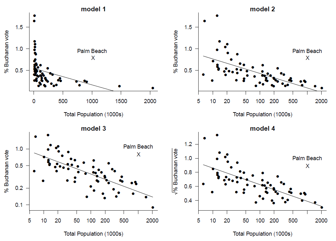
Figure 9.16: Least squares regression lines added to plots of the percentage of the vote for Buchanan against total population. Various transformations have been used.

Figures 9.17, 9.18, 9.19 and 9.20 show residual plots for each of these models.

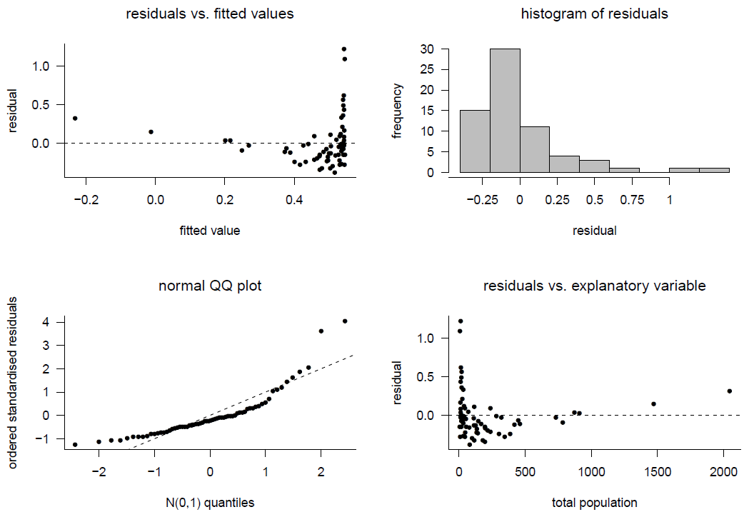
Figure 9.17: Model checking for model 1.

For Model 1 the plots of residuals against fitted values and residuals against Total Population indicate non-linearity and non-constant error variance. Given that the fit is so bad in these respects, it is pointless examining the histogram and normal QQ plot of the residuals. However, these plots indicate that the residuals look very unlike a sample from a normal distribution.

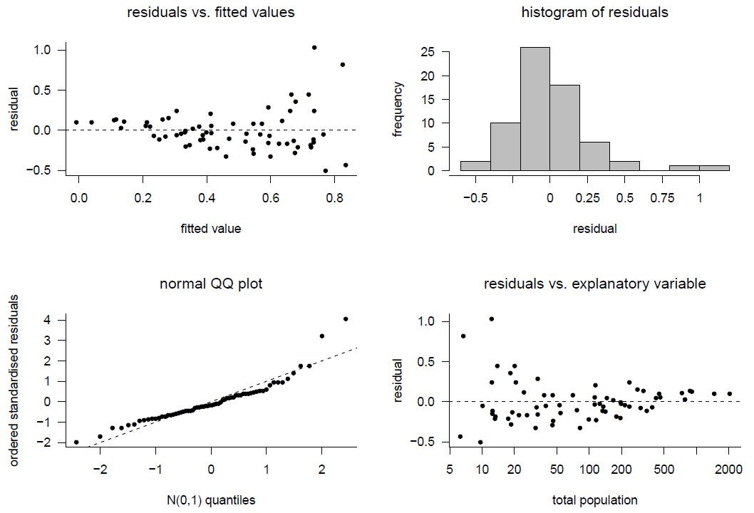
Figure 9.18: Model checking for model 2.

The general patterns in the plots for Model 2 are similar to those for Model 1, but the fit is improved compared to Model 1.

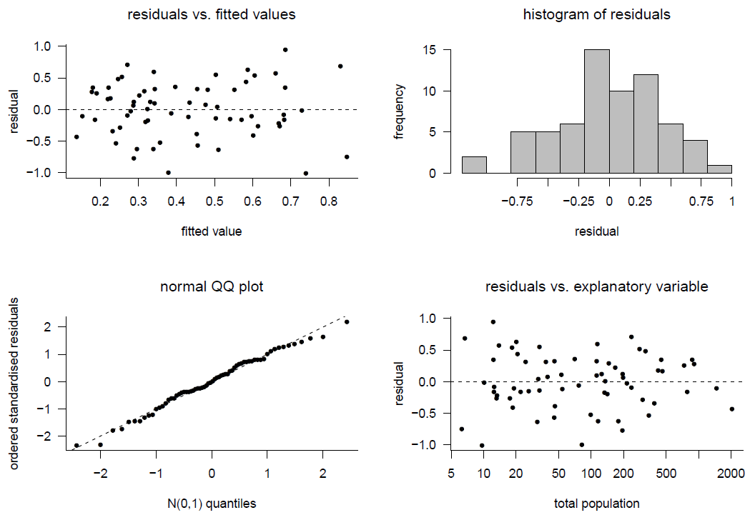
Figure 9.19: Model checking for model 3.

For Model 3 the plots of residuals against fitted values and against Total Population show a random scatter of points about the residual = 0 horizontal line. This is what we expect to see when the assumptions of linearity and constancy of error variance hold. In addition, the histogram and normal QQ plot of the residuals suggest that the residuals look like a sample from a normal distribution. This suggests that it would be reasonable to assume that the errors in the model are normally distributed.

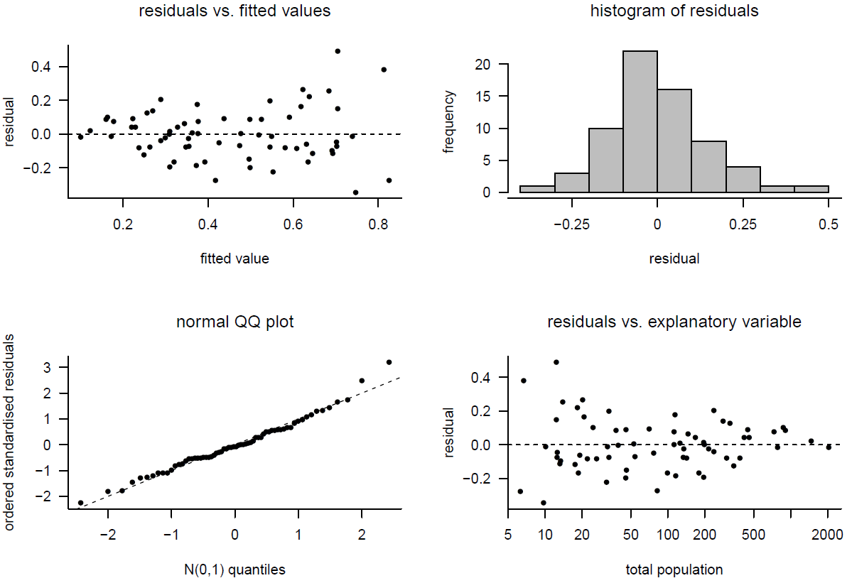
Figure 9.20: Model checking for model 4.

For Model 4 there is a slight suggestion in the plots of residuals against fitted values and residuals against Total Population that the error variance increases with the value of \(Y\), and hence decreases with the value of Total Population.

In summary, transformations may be used to

• make the relationship between two random variables closer to being linear;
• make the variance of a random variable \(Y\) closer to being constant in different groups, or for different values of another variable \(x\);
• make the distribution of a random variable more symmetric;
• make the distribution of a random variable (or an error term in a linear regression model) closer to being normal.

However, it may not be possible for a single transformation to achieve all the properties we want. For example, suppose that the relationship between \(Y\) and \(x\) is non-linear and that the variance of \(Y\) depends on the value of \(x\). We may find that

• the relationship between \(\sqrt{Y}\) and \(x\) is approximately linear, and
• the variance of \(\log Y\) is approximately constant for all values of \(x\).

If we wish to fit a linear regression model, after transforming \(Y\), a compromise is necessary.

9.4.1 Interpretation after transformation

If we use a transformation we should be careful to interpret the results carefully in light of the transformation used. Often we will want to report the results on the original scale of the data, rather than the transformed scale. We illustrate this using the 2000 US Presidential Election example, using Model 3: \[ \mbox{E}(\log Y \mid X=x) = \alpha+\beta\,\log x, \] where \(Y\) is the percentage of the vote obtained by Pat Buchanan and \(\log\) denotes the natural log, that is, log to the base \(e\). Again, we fit the model after excluding the observation from Palm Beach County. The least squares regression line is shown in the bottom left of Figure 9.16. The equation of this line is

\[ \widehat{\mbox{E}}(\log Y \mid X=x) = 0.4 - 0.3\,\log x, \]

that is, \(\hat{\alpha} = 0.4\) and \(\hat{\beta} = -0.3\).

This provides an estimate for the way that the mean of \(\log Y\) depends on \(x\). However, we may well be interested in \(Y\), not \(\log Y\). Recall from Section 5.3.4 that, some special cases aside, \(g[\mbox{E}(Y)] \neq \mbox{E}[g(Y)].\) In the current context,

\[ \log \mbox{E}(Y \mid X=x) \neq \mbox{E}(\log Y \mid X=x) \] or \[ \mbox{E}(Y \mid X=x) \neq \exp \left\{ \mbox{E}(\log Y \mid X=x) \right\}. \] Therefore, if we exponentiate the regression line then we do not obtain \(\mbox{E}(Y \mid X=x)\), at least not exactly.

We will consider two ways to tackle this problem.

Inferring \(\mbox{median}(Y \mid X = x).\) We assume that the error distribution is symmetric about 0, which implies that

\[ \mbox{E}(\log Y \mid X=x) = \mbox{median}(\log Y \mid X=x). \]

Consider a continuous random variable \(W\). If \(P(\log W \leq m) = 1/2\) then \(P(W \leq e^m) = 1/2\). If \(m\) is the median of \(\log W\) then \(e^m\) is the median of \(W\). Therefore,

\[ \mbox{median}(Y \mid X=x) = \exp \left\{ \mbox{median}(\log Y \mid X=x) \right\} = \exp \{ \alpha + \beta \, \log x\} = e^\alpha x^\beta. \]

This leads to the following estimate for the conditional median of \(Y\) given \(X = x\):

\[ \widehat{\mbox{median}}(Y \mid X=x) = e^{0.4 - 0.3\,\log x} = e^{0.4}\,x^{-0.3} = 1.5\,x^{-0.3}. \]

Based on this equation we estimate that if the population \(x\) doubles then the median of the percentage of the vote that Buchanan obtains is multiplied by \(2^{-0.3}=0.8\). Doubling the population is estimated to reduce the median of Buchanan’s vote by 20%, for example 5% would reduce to 4%. This provides an interpretation for the estimate \(\hat{\beta} = -0.3\). What about \(\hat{\alpha}=0.4\), or rather \(e^{0.4}=1.5\)? When \(x=1\), \[ \widehat{\mbox{median}}(Y \mid X=x) = 1.5. \] We estimate that in populations of size 1000 the median of Buchanan’s vote is 1.5% of the vote. However, The smallest population in the data is 6289 people, so we are extrapolating when we make this interpretation. It would be better to work with population recorded in units of 100,000. Then the intercept relates to a realistic population.

Inferring \(\mbox{E}(Y \mid X = x).\) We assume that the error distribution is normal. Suppose that \(Y\) and \(X\) are Buchanan’s percentage of the vote and the population size in an arbitrarily-chosen county. Given that \(X=x\) we have \[ \log Y = \alpha + \beta \log x + \epsilon, \] where \(\epsilon \sim N(0,\sigma^2)\). Therefore, \[ Y = e^\alpha x^\beta e^\epsilon. \] It can be shown that \(\mbox{E}\left(e^\epsilon\right)=e^{\sigma^2/2}\). Taking expectations gives

\[ \mbox{E}(Y \mid X=x) = \mbox{E}( e^\alpha x^\beta e^\epsilon) = e^\alpha x^\beta \mbox{E}\left( e^\epsilon \right) = e^\alpha \, x^\beta \, e^{\sigma^2/2}. \]

Therefore,

\[ \mbox{E}(Y \mid X = x) = e^{\sigma^2/2} \, \mbox{median}(Y \mid X = x). \]

Therefore, if the error variance \(\sigma^2\) is small then \(\mbox{E}(Y \mid X = x) \approx \mbox{median}(Y \mid X = x).\)

9.5 Over-fitting

We fitted a straight line model, \[ \mbox{E}(Y \mid X=x) = \alpha+\beta\,x, \] to Hubble’s data. Even if this model is true, we can (usually) obtain a better fit (smaller RSS) by fitting a quadratic model, \[\mbox{E}(Y \mid X=x) = \alpha+\beta\,x+\gamma\,x^2.\]

Extending this idea means that we can usually get closer and closer fits to the data by adding to the model a term in \(x^3\), a term in \(x^4\), and so on. Fitting a model with more than one explanatory variable is beyond the scope of STAT0002. However, in Figure 9.21 we show fits to Hubble’s data of polynomials of degree 2, 3, 4 and 8.

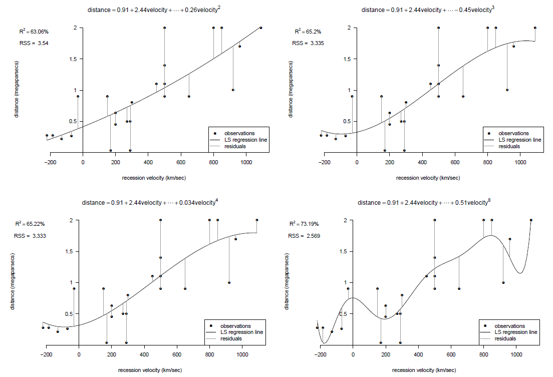
Figure 9.21: Fits of polynomial of degrees 2, 3, 4 and 8 to Hubble’s data.

As the degree of the polynomial increases the \(RSS\) decreases. Fitting a polynomial of degree 8 gives us a better fit (as judged by the values of RSS) than the linear fit. However, there are several reasons why using a high degree polynomial is a bad idea.

• Lack of sense. Fitting a very wiggly curve to these data doesn’t make sense: Hubble’s theory says that distance should be a linear function of velocity.
• Lack of understanding. Fitting a model which is too complicated doesn’t help our understanding the process which produced the data.
• Poor prediction. A fitted curve that is too complicated will tend to predict new values poorly, because the curve adapts too closely to the random wiggles of the data, rather than getting the general relationship between \(Y\) and \(x\) approximately correct. A model that fits existing data well doesn’t necessarily predict new observations well.

References

Freedman, Wendy L., Barry F. Madore, Brad K. Gibson, Laura Ferrarese, Daniel D. Kelson, Shoko Sakai, Jeremy R. Mould, et al. 2001. ‘Final Results from the Hubble Space Telescope Key Project to Measure the Hubble Constant’. The Astrophysical Journal 553 (1): 47–72. https://doi.org/10.1086/320638.

Hubble, Edwin. 1929. ‘A Relation Between Distance and Radial Velocity Among Extra-Galactic Nebulae’. Proceedings of the National Academy of Sciences 15 (3): 168–73. https://doi.org/10.1073/pnas.15.3.168.