Chapter 5 Random variables

Example. We return to the space shuttle example.

Consider what happens to the O-rings on a particular test flight, at a particular temperature. A given O-ring either is damaged (shows signs of thermal distress) or it is not damaged. Let \(D\) denote the event that an O-ring is damaged and \(\bar{D}\) the event that it is not damaged. If we consider all 6 O-rings, there are many possible outcomes in the sample space, \(2^6=64\), in fact: \[ S= \{DDDDDD\}, \{DDDDD\bar{D}\}, \ldots, \{D\bar{D}\bar{D}\bar{D}\bar{D}\bar{D}\}, \{\bar{D}\bar{D}\bar{D}\bar{D}\bar{D}\bar{D}\}. \] Suppose that we are not interested in which particular O-rings were damaged, just the total number \(N\) of damaged O-rings. The possible values for \(N\) are 0,1,2,3,4,5,6.

Each outcome in \(S\) gives a value for \(N\) in {0,1,2,3,4,5,6}:

\(\{DDDDDD\}\) gives \(N=6\),

\(\{DDDDD\bar{D}\}\) gives \(N=5\),

\(\{DDDD\bar{D}D\}\) gives \(N=5\),

\(\vdots\)

\(\{\bar{D}\bar{D}\bar{D}\bar{D}\bar{D}\bar{D}\}\) gives \(N=0\).

By defining \(N\) to be the total number of damaged O-rings, we have moved from considering outcomes to considering a variable with a numerical value. \(N\) is a real-valued function on the sample space \(S\), that is, \(N\) maps each outcome in \(S\) to a real number. \(N\) is a rule that assigns a real number to every outcome \(s\) in \(S\). Since the outcomes in \(S\) are random the variable \(N\) is also random, and we can assign probabilities to its possible values, that is, \(P(N=0), P(N=1)\) and so on.

\(N\) is a random variable. In fact, if we assume that O-rings are damaged independently of each other and each O-ring has the same probability \(p\) of being damaged, \(N\) is a random variable with a special name. It is a binomial random variable with parameters 6 and \(p\). We will consider binomial random variables in more detail in Section 6.3.

Notation. We denote random variables by upper case letters, for example, \(N, X, Y, Z\). Once we have observed the value of a random variable it is no longer random: it is equal to a particular numeric value. To make this clear we denote sample values of r.v.s. by lower case letters, for example, \(n, x, y, z\) and write \(N=n, X=x\) and so on. Thus, \(P(X=x)\) is the probability that the random variable \(X\) has the value \(x\).

5.1 Discrete random variables

Definition. A discrete random variable is a random variable that can take only a finite, or countably infinite, number of values.

An example of a countably infinite set of values is {0,1,2,3, …}. The random variable \(N\) in the space shuttle example takes a finite number of values: 0,1,2,3,4,5,6. Therefore \(N\) is a discrete random variable.

Definition. Let \(X\) be a discrete random variable. The probability mass function (p.m.f.) \(p_X(x)\), or simply \(p(x)\), of \(X\) is \[ p_X(x) = P(X=x), \qquad \mbox{for $x$ in the support of $X$}. \]

The p.m.f. of \(X\) tells us the probability with which \(X\) takes any particular value \(x\). The support of \(X\) is the set of values that it is possible for \(X\) to take. It is very important to write this down every time you write down a p.m.f.. A discrete random variable is completely specified by its probability mass function.

Properties of p.m.f.s

Let \(X\) take values \(x_1, x_2,\ldots.\) Then

1. \(p_X(x_i) \geq 0\), for all \(i\),
2. \(\displaystyle\sum_i p_X(x_i) = 1\).

Note: 1. is true because the \(p_X(x_i)\)s are probabilities; 2. is true because summing over the \(x_i\)s is equivalent to summing over the sample space of outcomes.

Definition. The cumulative distribution function (c.d.f.) of a random variable \(X\) is \[ F_X(x) = P(X \leq x), \qquad \mbox{for} -\infty < x < \infty. \]

Relationship between the c.d.f. and p.m.f. of a discrete random variable. For a discrete random variable: \[ F_X(x) = P(X \leq x) = \sum_{x_i \leq x} P(X = x_i). \] Therefore, assuming for the moment that the random variable takes only integer values, \[ P(X=x) = P(X \leq x) - P(X \leq x-1) = F_X(x) - F_X(x-1) \] for any integer \(x\)

5.2 Continuous random variables

Example. We return to the Oxford birth times example.

The top plot in Figure 5.1 shows a histogram of the 95 birth times. The variable of interest in this example is a time. Time is a continuous variable: in principle, the times in this dataset could take any positive real value, uncountably many values. In practice, these times have been recorded discretely, in units of 1/10 of an hour or 1/4 of an hour.

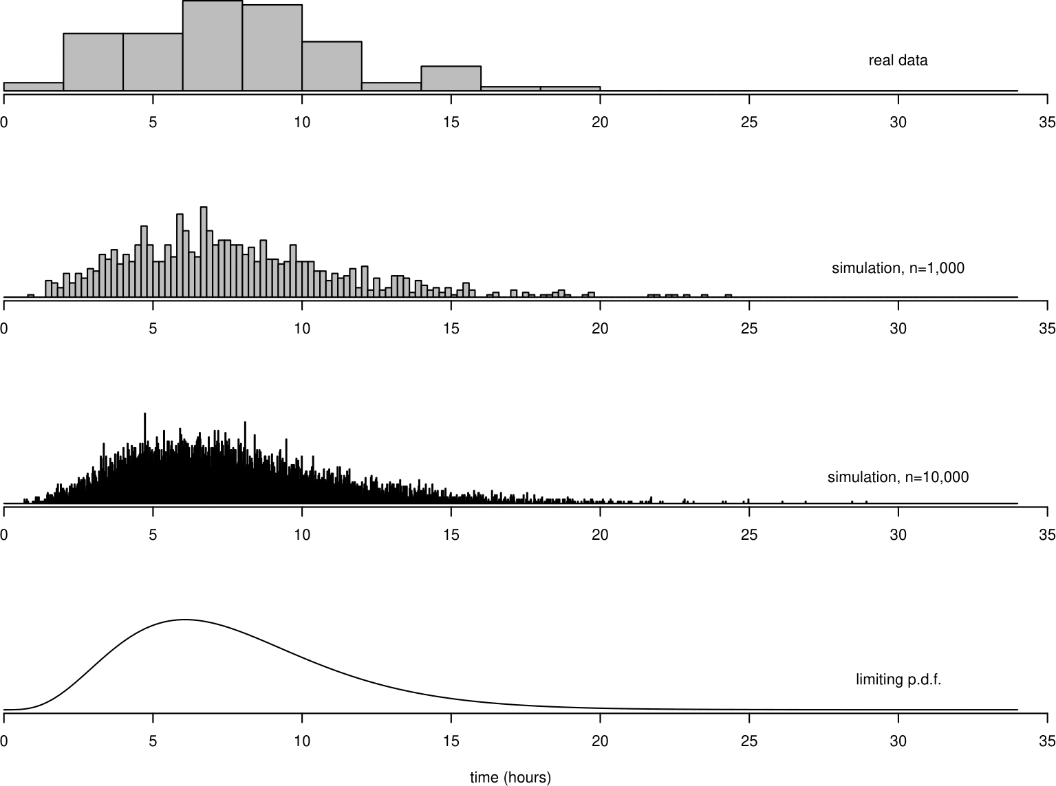
Figure 5.1: Top: histogram of the Oxford birth durations. Second from top: histogram of 1,000 values simulated from a distribution fitted to the data. Second from bottom: similarly for 10,000 simulated values. Bottom: p.d.f. of the distribution fitted to the Oxford birth times data.

Suppose that we continue to collect data on birth duration from this hospital, and, as new observations arrive, we add them to the top histogram in Figure 5.1. We imagine that the times are recorded continuously. As the number of observations \(n\) increases we decrease the bin width of the histogram. As \(n\) increases to infinity the bin width shrinks to zero and the histogram tends to a smooth continuous curve.

This is shown in the bottom 3 plots in Figure 5.1. The extra data are not real. They are data I have simulated, using a computer, to have a distribution with a similar shape to the histogram of the real data.

Let \(T\) denote the time, in hours, that a woman arriving at the hospital takes to give birth. The smooth continuous curve at the bottom of Figure 5.1 is called the probability density function (p.d.f.) \(f_T(t)\) of the random variable \(T\). Since the total area of the rectangles in a histogram is equal to 1, the area \(\int_{-\infty}^{\infty} f_T(t) \, \mathrm{d}t\) under the p.d.f. \(f_T(t)\) is equal to 1.

Definition. A probability density function (p.d.f.) is a function \(f_{X}(x)\), or simply \(f(x)\), such that

1. \(f_X(x) \geq 0\), for \(-\infty < x < \infty\);
2. \(\displaystyle\int_{-\infty}^{\infty} f_X(x) \, \mathrm{d}x = 1\).

Therefore, p.d.f.s are always non-negative and integrate to 1. The support of a continuous random variable is the set of values for which the p.d.f. is positive. Suppose that we wish to find \(P(4 < T \leq 12)\). To find the proportion of times between 4 and 12 using a histogram, we sum the areas of all bins between 4 and 12, that is, we find the area shaded in the histogram in Figure 5.2. To do this using the p.d.f. we do effectively the same thing: we find the area under the p.d.f. \(f_T(t)\) between 4 and 12. Since \(f_T(t)\) is a smooth continuous curve, (that is, the bin widths are zero) we integrate \(f_T(t)\) between 4 and 12.

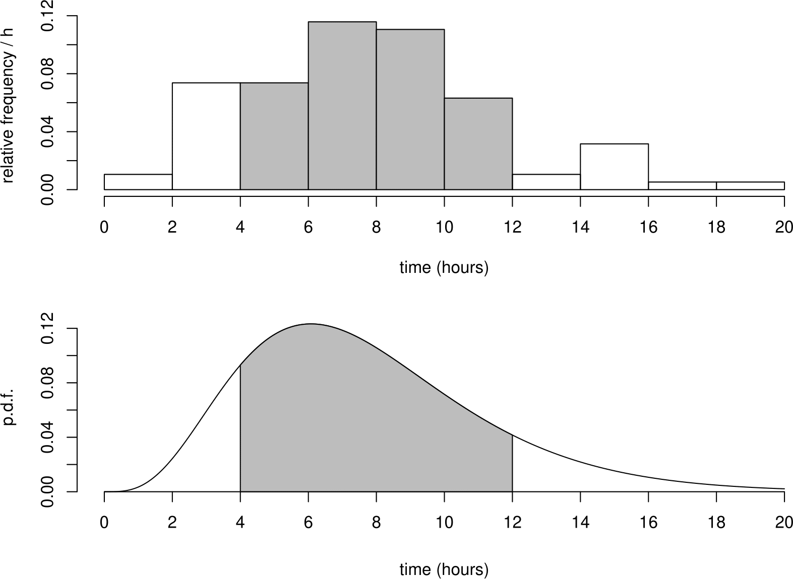
Figure 5.2: Top: histogram of the Oxford birth durations. Bottom: p.d.f. of the distribution fitted to the Oxford birth duration data.

Therefore \[ P(4 < T \leq 12) = \displaystyle\int_4^{12} f_T(t) \,\mathrm{d}t = F_T(12)-F_T(4). \]

More generally, \[ P(a < T \leq b) = \displaystyle\int_a^b f_T(t) \,\mathrm{d}t = F_T(b)-F_T(a). \]

Definition. A random variable \(X\) is a continuous random variable if there exists a p.d.f. \(f_X(x)\) such that \[ P(a < X \leq b) = \int_{a}^{b} f_X(x) \,\mathrm{d}x, \] for all \(a\) and \(b\) such that \(a < b\).

Figure 5.3 illustrates the properties of a p.d.f..

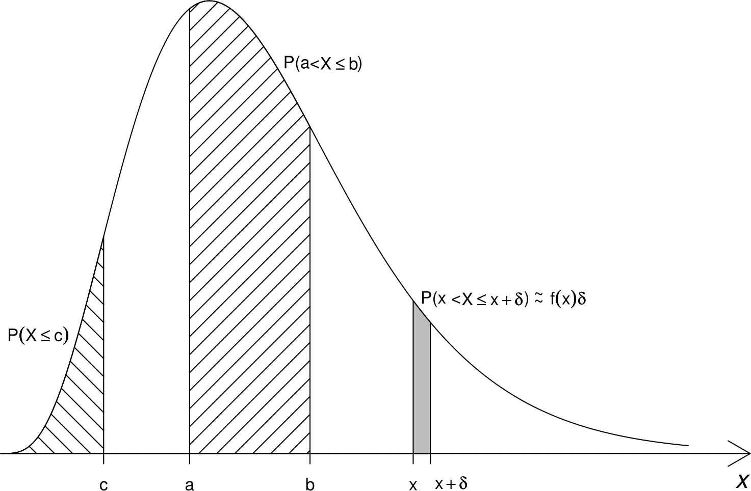
Figure 5.3: Properties of a p.d.f.. The areas that correspond to the probability that a random variable takes a value in a given interval are shaded.

Notes

• It is very important to appreciate that \(f_X(x)\) is not a probability: it does not give \(P(X=x)\). In fact \(P(X=x)=0\): the probability that a continuous random variable \(X\) takes the value \(x\) is zero.
• Indeed, it is possible for a p.d.f. to be greater than 1. Consider a continuous random variable \(X\) with p.d.f. \[ f_X(x) = \left\{ \begin{array}{ll} 2\,(1-x) & \,0 \leq x \leq 1, \\ 0 & \,\mbox{otherwise}.\end{array}\right. \] For this random variable \(f_X(x)>1\) for any \(x \in [0, 1/2)\) .
• Since, for any \(x \in \mathbb{R}\), \(P(X=x)=0\) \[ P(a < X \leq b) = P(a \leq X \leq b) = P(a \leq X < b) = P(a < X < b). \]
• \(f_X(x)\) is a probability density. The probability that \(X\) lies in a very small interval of length \(\delta\) near \(x\) is approximately \(f_X(x) \delta\). For the p.d.f. at the bottom of Figure 5.1, \(f_T(6) > f_T(12)\), indicating that a randomly chosen woman is more likely to spend approximately 6 hours giving birth than approximately 12 hours.

Relationship between the c.d.f. and p.d.f. of a continuous random variable. For a continuous random variable \[ F_X(x) = P(X \leq x) = \int_{-\infty}^x f_X(u) \,\mathrm{d}u. \] Therefore, \[ f_X(x) = \frac{\mathrm{d}}{\mathrm{d}x} F_X(x). \]

5.3 Expectation

The expectation of a random variable is a measure of the location of its distribution.

5.3.1 Expectation of a discrete random variable

Example. We return to the space shuttle example.

Again we consider test flights conducted at a particular temperature, say 53\(^\circ\)F. Suppose that NASA are able to conduct a very large number \(n\) of test flights at 53\(^\circ\)F, producing a sample \(x_1,\ldots,x_n\) of numbers of damaged O-rings.

Let \(n(x)\) be the number of test flights on which \(x\) of the 6 O-rings were damaged. We can write the sample mean \(\bar{x}\) of \(x_1,\ldots,x_n\) as \[\begin{eqnarray*} \bar{x} &=& \frac{0 \times n(0) + 1 \times n(1) + \cdots + 6 \times n(6)}{n}, \\ &=& \sum_{x=0}^6 x\,\frac{n(x)}{n}. \end{eqnarray*}\] As the sample size \(n\) increases to infinity, the sample proportion \(n(x)/n\) tends to \(P(X=x)\), for \(x=0,1,\ldots,6\). Therefore, in the limit as \(n \rightarrow \infty\), \(\bar{x}\) tends to \[\begin{eqnarray} \sum_{x=0}^6 x\,P(X=x). \tag{5.1} \end{eqnarray}\] This is known as the mean of the probability distribution of \(X\). It is a measure of the location of the distribution.

The quantity in equation (5.1) is the value of the sample mean \(\bar{x}\) that we would expect to get from a very large sample. Therefore it is often called the expectation or expected value of the random variable \(X\) and it is denoted \(\mathrm{E}(X)\).

Definition. The expectation (or expected value or mean) \(\mathrm{E}(X)\) of a discrete random variable \(X\) is given by \[\begin{eqnarray} \mathrm{E}(X) &=& \sum_x x\,P(X=x). \tag{5.2} \end{eqnarray}\] This is a weighted average of the values that \(X\) can take, each value being weighted by \(P(X=x)\).

Note:

• We often write \(\mu\) or \(\mu_X\) for \(\mathrm{E}(X)\).
• Units: the units of \(\mathrm{E}(X)\) are the same as those of \(X\). For example, if \(X\) is measured in hours then \(\mathrm{E}(X)\) is measured in hours.
• \(\mathrm{E}(X)\) exists only if \(\sum_x |x|\,P(X=x) < \infty\). If the number of values \(X\) can take is finite then \(\mathrm{E}(X)\) will always exist.

5.3.2 Expectation of a continuous random variable

We can define the expectation of a continuous random variable in a similar way to a discrete random variable, replacing summation with integration.

Definition. The expectation \(\mathrm{E}(X)\) of a continuous random variable \(X\) is given by \[\begin{eqnarray} \mathrm{E}(X) = \int_{-\infty}^{\infty} x\,f_X(x) \,\mathrm{d}x. \tag{5.3} \end{eqnarray}\] Note:

• Like the discrete case, this is a weighted average of the values that \(X\) can take, but now each value is weighted by the p.d.f. \(f_X(x)\).
• The range of integration in equation (5.3) is over the whole real line but, in practice, integration will be over the range of possible values of \(X\).
• \(\mathrm{E}(X)\) exists only if \(\int_{-\infty}^{\infty} |x|\,f_X(x) \,\mathrm{d}x < \infty\).

5.3.3 Properties of \(\mathrm{E}(X)\)

If \(a\) and \(b\) are constants then \[ \mathrm{E}(a\,X+b) = a\,\mathrm{E}(X)+b. \] This makes sense. If we multiply all observations by \(a\) their mean will also be multiplied by \(a\). If we add \(b\) to all observations their mean will be increased by \(b\), that is, the distribution of \(X\) shifts up by \(b\).

• If \(X \geq 0\) then \(\mathrm{E}(X) \geq 0\).
• If \(X\) is a constant \(c\), that is, \(P(X=c)=1\) then \(\mathrm{E}(X)=c\).
• It can be shown that \[ \mathrm{E}(X_1 + X_2 + \cdots + X_n) = \mathrm{E}(X_1) + \mathrm{E}(X_2) + \cdots + \mathrm{E}(X_n). \]

5.3.4 The expectation of \(g(X)\)

Suppose that \(Y=g(X)\) is a function of of \(X\), such as \(aX+b\), \(X^2\) or \(\log X\). Then \(Y\) is also a random variable. If we find the p.m.f (if \(Y\) is discrete) or p.d.f. (if \(Y\) is continuous) of \(Y\) then we can find the expectation of \(Y\) using equation (5.2) or (5.3) as appropriate. Alternatively, and often more easily, we can use

\[\begin{equation} \mathrm{E}(Y) = \mathrm{E}[g(X)] = \begin{cases} \displaystyle\sum_x g(x)\,P(X=x) & \text{if } X \text{ is discrete}, \\ \int_{-\infty}^{\infty} g(x)\,f_X(x) \,\mathrm{d}x & \text{if } X \text{ is continuous}. \end{cases} \tag{5.4} \end{equation}\]

Note: for a non-linear function \(g(X)\), it is usually the case that \[ \mathrm{E}[g(X)] \neq g[\mathrm{E}(X)] \] although there are exceptions.

5.4 Variance

The variance of a random variable is a measure of the spread of its distribution.

5.4.1 Variance of a discrete random variable

Example. We return the space shuttle example.

As before we let \(n(x)\) be the number of test flights on which \(x\) of the 6 O-rings were damaged. We saw in Section 2.3.2 that a measure of the spread of a sample \(x_1,\ldots,x_n\) is the sample variance \(s_X^2\) which, in this example, can be written as

\[\begin{eqnarray*} s_X^2 &=& \frac{1}{n-1}\,\left\{ (0-\bar{x})^2\,n(0)+(1-\bar{x})^2\,n(1)+\cdots+(6-\bar{x})^2\,n(6) \right\}, \\ &=& \sum_{x=0}^6 (x-\bar{x})^2\,\frac{n(x)}{n-1}. \end{eqnarray*}\] As the sample size \(n\) increases to infinity, \(\frac{n(x)}{n-1}\) tends to \(P(X=x)\), for \(x=0,1,\ldots,6\) and \(\bar{x}\) tends to \(\mu\)=\(\mathrm{E}(X)\).

Therefore, as \(n \rightarrow \infty\), \(s_X^2\) tends to

\[\begin{equation} \sum_{x=0}^6 (x-\mu)^2\,P(X=x). \tag{5.5} \end{equation}\]

This is known as the variance of the probability distribution of \(X\). It is a measure of the spread of the distribution. The quantity in equation (5.5) is the value of the sample variance \(s_X^2\) that we would expect to get from a very large sample.

Definition. The variance \(\mathrm{var}(X)\) of a discrete random variable \(X\) with mean \(\mathrm{E}(X)=\mu\) is given by

\[\begin{equation} \mathrm{var}(X) = \sum_x\,(x-\mu)^2\,P(X=x). \tag{5.6} \end{equation}\]

This is a weighted average of the squared differences between the values that \(X\) can take and its mean \(\mu\), each value being weighted by \(P(X=x)\).

A variance can be infinite. If the number of values that \(X\) can take is finite then \(\mathrm{var}(X)\) will always be finite.

5.4.2 Variance of a continuous random variable

We can define the variance of a continuous random variable in a similar way to a discrete random variable, replacing summation with integration.

Definition. The variance \(\mathrm{var}(X)\) of a continuous random variable \(X\) with mean \(\mathrm{E}(X)=\mu\) is given by

\[\begin{equation} \mathrm{var}(X) = \int_{-\infty}^{\infty} (x-\mu)^2 f_X(x) \,\mathrm{d}x. \tag{5.7} \end{equation}\]

5.4.3 Variance and standard deviation

Definition. Let \(X\) be a random variable with \(\mathrm{E}(X)=\mu\). The variance \(\mathrm{var}(X)\) is given by \[ \mathrm{var}(X) = \mathrm{E}\left[(X-\mu)^2\right]. \] This follows from equations (5.6) and (5.7) and the expression in equation (5.4) for the expectation of a function \(g(X)\) of a random variable \(X\).

There is an alternative way to calculate \(\mathrm{var}(X)\): \[ \mathrm{var}(X) = \mathrm{E}\left(X^2\right) - [\mathrm{E}(X)]^2. \]

Exercise. Prove this.

Definition. The standard deviation sd\((X)\) of \(X\) is given by sd(\(X\))=\(+\sqrt{\mathrm{var}(X)}\).

Notes on \(\mathrm{var}(X)\) and sd(\(X\)):

• \(\mathrm{var}(X) \geq 0\) and \(\mathrm{sd}(X) \geq 0\). Variances and standard deviations cannot be negative.
  
• The units of \(\mathrm{var}(X)\) are the square of those of \(X\). For example, if \(X\) is measured in hours then \(\mathrm{var}(X)\) is measured in hours\(^2\) (and sd(\(X\)) is measured in hours). The units of \(\mathrm{sd}(X)\) are the same as those of \(X\).
• We often write \(\sigma^2\) or \(\sigma_X^2\) for \(\mathrm{var}(X)\) and \(\sigma\) or \(\sigma_X\) for \(\mathrm{sd}(X)\).
• \(\mathrm{var}(X)\) exists only if \(\mu\) exists.

5.4.4 Properties of \(\mathrm{var}(X)\)

• If \(a\) and \(b\) are constants then \[ \mathrm{var}(a\,X+b) = a^2\,\mathrm{var}(X). \] This makes sense. If we multiply all observations by \(a\) their variance, which is measured square units, will be multiplied by \(a^2\). If we add \(b\) to all observations their variance will be unchanged because the distribution simply shifts up by \(b\) and its spread is unaffected.
• If \(X\) is a constant \(c\), that is, \(P(X=c)=1\) then \(\mathrm{var}(X)=0\): the distribution of \(X\) has zero spread.
• It can also be shown that if the random variables \(X_1, X_2, \ldots X_n\) are independent (see An Aside below) then

\[\begin{equation} \mathrm{var}(X_1 + X_2 + \cdots + X_n) = \mathrm{var}(X_1) + \mathrm{var}(X_2) + \cdots + \mathrm{var}(X_n). \tag{5.8} \end{equation}\]

Note. Independence is sufficient for this result to hold but it is not necessary. Taking \(n=2\) as an example, in generality we have \[ \mathrm{var}(X_1 + X_2) = \mathrm{var}(X_1) + \mathrm{var}(X_2) + 2\,\mathrm{cov}(X_1,X_2), \] where \(\mathrm{cov}(X_1,X_2)\) is the covariance between the random variables \(X_1\) and \(X_2\). Covariance is a measure of the strength of linear association. If \(X_1\) and \(X_2\) are independent (have no association of any kind) then \(\mathrm{cov}(X_1,X_2)=0\), because they have no linear association. However, it is possible for \(X_1\) and \(X_2\) to be dependent but \(\mathrm{cov}(X_1,X_2)=0\), because, although they have some kind of association, they have no linear association. Thus, independence is a stronger requirement than zero covariance.

Returning to general \(n\) we have \[ \mathrm{var}(X_1 + X_2 + \cdots + X_n) = \mathrm{var}(X_1) + \mathrm{var}(X_2) + \cdots + \mathrm{var}(X_n) + 2 \mathop{\sum\sum}_{i < j} \mathrm{cov}(X_i,X_j). \] If \(\mathrm{cov}(X_i,X_j)=0\) for all \(i < j\) then equation (5.8) holds. We will study covariance, and its standardised form correlation, in Chapter 10.

5.4.4.1 An aside

(This is beyond the scope of STAT0002. It is included here for completeness and in case you are interested.) To consider more formally what it means for random variables \(X_1, ..., X_n\) to be independent we define their joint c.d.f. \(F_{X_1, ..., X_n}(x_1, ..., x_n) = P(X_1 \leq x_1, ..., X_n \leq x_n)\). The random variables \(X_1, ..., X_n\) are (mutually) independent if \(F_{X_1, ..., X_n}(x_1, ..., x_n) = F_{X_1}(x_1) \times \cdots \times F_{X_n}(x_n)\), that is, \(P(X_1 \leq x_1, ..., X_n \leq x_n) = P(X_1 \leq x_1) \times \cdots \times P(X_n \leq x_n)\), for any set of values \((x_1, .., x_n)\). The random variables \(X_1, ..., X_n\) are pairwise independent if, \(F_{X_i, X_j}(x_i, x_j) = F_{X_i}(x_i) F_{X_j}(x_j)\), that is, \(P(X_i \leq x_i, X_j \leq x_j) = P(X_i \leq x_i) P(X_j \leq x_j)\), for every pair \((X_i, X_j)\) of variables that we could select from \(X_1, ..., X_n\) and for any pair of values \((x_i, x_j)\).

5.5 Other measures of location

5.5.1 The median of a random variable

Recall that the sample median of a set of observations is the middle observation when the observations are arranged in order of size. We define the median of a random variable \(X\) as a value, median(\(X\)), such that

\[ P(X < \mathrm{median}(X)) \leq \frac12 \leq P(X \leq \mathrm{median}(X)). \]

In other words, \(\mathrm{median}(X)\) is a value where a plot of the c.d.f. \(F_X(x)=P(X \leq x)\) hits \(1/2\).

For a continuous random variable \(X\) we have \[ F_X(\mathrm{median}(X)) = P(X \leq \mathrm{median}(X)) =\frac12. \] and a median will divide the distribution into two parts, each with probability 1/2: \[ P(X < \mathrm{median}(X)) = P(X > \mathrm{median}(X)) = \frac12. \]

This will not necessarily hold for a discrete distribution. For example, suppose that \[ P(X=0)=\frac16, \qquad P(X=1)=\frac12, \qquad P(X=2)=\frac13. \]

Then \[\begin{eqnarray*} F_X(x) = P(X \leq x) = \left\{\begin{array}{ll} 0 & \mbox{for } x <0, \\ \frac16 & \mbox{for } 0 \leq x < 1, \\ \frac23 & \mbox{for } 1 \leq x < 2, \\ 1 & \mbox{for } x \geq 2, \end{array}\right. \end{eqnarray*}\]

Figure 5.4 is a plot of the c.d.f. of this discrete random variable.

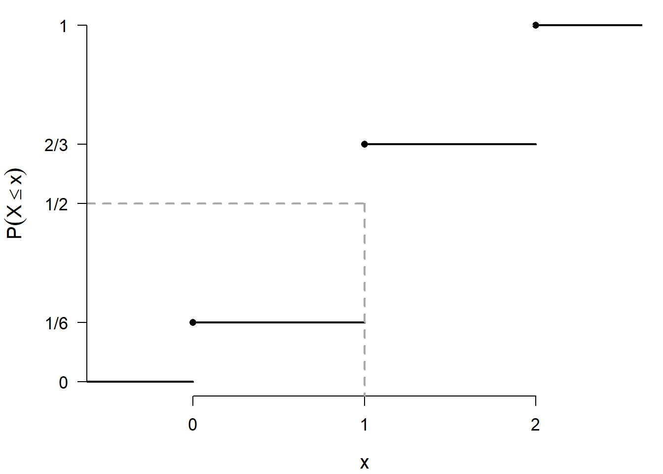
Figure 5.4: Plot of the c.d.f. of a discrete random variable that takes the values {0, 1, 2} with respective probabilities {1/6, 1/2, 1/3}. The dashed lines indicate the location of the median (1).

Therefore, \(\mathrm{median}(X) = 1\). However, \(P(X<1)=\frac16\) and \(P(X>1)=\frac13\).

5.5.2 The mode of a random variable

Recall that the sample mode of categorical or discrete data is the value (or values) which occurs most often. We define the mode, mode(\(X\)), of a random variable as follows.

For a discrete random variable \(X\), the mode is the value which has the highest probability of occurring: \(P(X=\mathrm{mode}(X))\) will be larger than for any other value \(X\) can have. In other words, \(\mathrm{mode}(X)\) is the value at which the p.m.f. is maximised.

For a continuous random variable \(X\), the mode is the value at which the p.d.f. is maximised. If the maximum occurs at a turning point of \(f_X(x)\) then it can be found by solving the equation \[ \frac{\mathrm{d}}{\mathrm{d}x} f_X(x) = 0, \] and checking that you have indeed found a maximum.

5.6 Quantiles

To keep things simple we consider a continuous random variable \(X\). For \(0 < p < 1\), a \(100p\%\) quantile of \(X\) is defined to be a value \(x_p\) such that \[ F_X(x_p)=P(X \leq x_p) = p. \] Another way to express this is to say that \(x_p\) is \(F_X^{-1}(p)\), where \(F_X^{-1}\) is the inverse c.d.f. of \(X\). The inverse c.d.f. \(F_X^{-1}\) is also called the quantile function \(Q\) of \(X\), so we could write \(x_p = Q(p)\).

Thus, \(x_{1/4}=F_X^{-1}(1/4)\) is the lower quartile of \(X\), \(x_{1/2}=F_X^{-1}(1/2)\) is the median of \(X\) and \(x_{3/4}=F_X^{-1}(3/4)\) is the upper quartile of \(X\).

The inter-quartile range is \(x_{3/4}-x_{1/4}=F_X^{-1}(3/4)-F_X^{-1}(1/4)\), which is a measure of spread.

5.7 Measures of shape

The moment coefficient of skewness of a random variable \(X\) with mean \(\mu\) and standard deviation \(\sigma\) is given by \[ \mathrm{E}\left[\left(\frac{X - \mu}{\sigma}\right)^3\right] = \displaystyle\frac{\mathrm{E}\left[\left(X- \mu\right)^3\right]}{\sigma^3}, \] provided that \(\mathrm{E}[\left(X- \mu\right)^3]\) exists.

The quartile skewness of a random variable \(X\) with c.d.f \(F_X(x)\) is given by \[ \frac{(x_{3/4}-x_{1/2}) - (x_{1/2}-x_{1/4})}{x_{3/4}-x_{1/4}} = \frac{[F^{-1}_X(3/4) - F^{-1}_X(1/2)] - [F^{-1}_X(1/2) - F^{-1}_X(1/4)]}{F^{-1}_X(3/4) - F^{-1}_X(1/4)}. \]