Chapter 3 Probability
Most people have heard the word probability used in connection with a random experiment, that is, an experiment whose outcome cannot be predicted with certainty, such as tossing a coin, tossing dice, dealing cards etc. We start by considering a criminal case in which fundamental ideas surrounding the use of probability were hugely important. Then we study the concept of probability using the traditional simple example of tossing a coin.
3.1 Misleading statistical evidence in cot death trials
In recent years there have been three high-profile criminal cases in which a mother has been put on trial for the murder of a her babies. In each case the medical evidence against the woman was weak and the prosecution relied heavily on statistical arguments to make their case. However, these arguments were not made by a statistician, but by a medical expert witness: Professor Sir Roy Meadows. However, there were two problems with Professor Meadows’ evidence: firstly, it contained serious statistical errors; and secondly, it was presented in a way which is likely to be misinterpreted by a jury. To illustrate the error we consider the case of Sally Clark.
Sally Clark’s first child died unexpectedly in 1996 at the age of 3 months. Sally was the only person in the house at the time. There was evidence of a respiratory infection and the death was recorded as natural; a case of Sudden Infant Death Syndrome (SIDS), or cot death. In 1998 Sally’s second child died in similar circumstances at the age of 2 months. Sally was then charged with the murder of both babies. There was some medical evidence to suggest that the second baby could have been smothered, although this could be explained by an attempt at resuscitation.
It appeared that the decision to charge Sally was based partly on the reasoning that cot death is quite rare so having two cot deaths in the same family must be very unlikely indeed. This is the basis of Professor Meadows’ assertion that: “One cot death is a tragedy, two cot deaths is suspicious and, until the contrary is proved, three cot deaths is murder.”. At her trial in 1999 Sally Clark was found guilty of murder and sentenced to life imprisonment.
Professor Meadows’ statistical evidence
At Sally Clark’s trial in 1999 Professor Meadows claimed that, in a family like Sally’s (affluent, non-smoking with a mother aged over 26), the chance of two cot deaths is 1 in 73 million, that is, a probability of 1/73,000,000 \(\approx\) 0.000000014. Professor Meadows had calculated this value based on a study which had estimated the probability of one cot death in a family like Sally’s to be 1 in 8543, that is, 1 cot death occurs for every 8543 of such families.
Professor Meadows had then performed the calculation \[\frac{1}{8543}\times\frac{1}{8543}=\frac{1}{72,982,849}\approx\frac{1}{73,000,000}.\]
There are problems with this evidence, both with this calculation and with the idea that this apparently small number provides evidence of guilt.
Can you identify these problems?
3.2 Relative frequency definition of probability
Example: tossing a coin
If you toss a coin, the outcome (the side on top when the coin falls to the ground) is either a Head (\(H\)) or a Tail (\(T\)). Suppose that you toss the coin a large number of times. Unless you are very skillful the outcome of each toss depends on chance. Therefore, if you toss the coin repeatedly, the exact sequence of \(H\)s and \(T\)s is not predictable with certainty in advance. This is usually the case with any experiment. Even if we try very hard to repeat an experiment under exactly the same conditions, there is a certain amount of variability in the results which we cannot explain, but we must accept. The experiment is a random experiment.
Nevertheless, if the coin is fair (equally balanced), and it is tossed fairly, we might expect the long run proportion, or relative frequency, of \(H\)s to settle down to 1/2. However, the only way to find out whether this is true is to toss a coin repeatedly, forever, and calculate the proportion of tosses on which \(H\) is the outcome. It is not possible, in practice, for any experiment to be repeated forever.
However, a South African statistician Jon Kerrich managed to toss a coin 10,000 times while imprisoned in Denmark during World War II. At the end of his effort he had recorded 5067 Heads and 4933 Tails. Figure 3.1 shows how the proportion of heads Kerrich threw changed as the number of tosses increased.
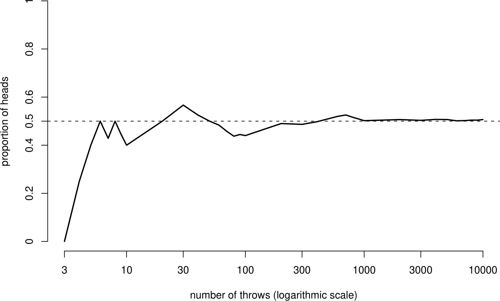
Figure 3.1: The proportion of heads in a sequence of 10,000 coin tosses. Kerrich (1946).
Initially the proportion of heads fluctuates greatly but begins to settle down as the number of tosses increases. After 10,000 tosses the relative frequency of Head is 5067/10,000=0.5067. We might suppose that if Kerrich were able to continue his experiment forever, the proportion of heads would tend to a limiting value which would be very near, if not exactly, 1/2. This hypothetical limiting value is the probability of heads and is denoted by \(P(H)\).
Looking at this slightly more formally
The coin-tossing example motivates the relative frequency or frequentist definition of the probability of an event; namely
the relative frequency with which the event occurs in the long run;
or, in other words,
the proportion of times that the event would occur in an infinite number of identical repeated experiments.
Suppose that we toss a coin \(n\) times. If the coin is fair, and is tossed fairly, then it is reasonable to suppose that \[\text{the relative frequency of } H \,\,=\,\, \frac{\text{number of times } H \text{ occurs}}{n},\] tends to 1/2 as \(n\) gets larger. We say that the event \(H\) has probability 1/2, or \(P(H)=1/2\).
More generally, consider some event \(E\) based on the outcomes of an experiment. Suppose that the experiment can, in principle, be repeated, under exactly the same conditions, forever. Let \(n(E)\) denote the number of times that the event \(E\) would occur in \(n\) experiments.
We suppose that \[\text{the relative frequency of $E$} \,=\, \frac{n(E)}{n} \,\longrightarrow\, P(E)\,, \,\, \text{as }n \longrightarrow \infty.\] So, the probability \(P(E)\) of the event \(E\) is defined as the limiting value of \(n(E)/n\) as \(n \rightarrow \infty\). That is, \[\begin{equation} P(E) \,\,=\,\, \mathop {\mathrm{limit}}\limits_{n \rightarrow \infty}\,\frac{n(E)}{n}, \tag{3.1} \end{equation}\] supposing that this limit exists. (Note: I have written ‘limit’ and not ‘lim’ because this is not a limit in the usual mathematical sense.)
In order to satisfy ourselves that the probability of an event exists, we do not need to repeat an experiment an infinite number of times, or even be able to. All we need to do is imagine the experiment being performed repeatedly. An event with probability 0.75, say, would be expected to occur 75 times out of 100 in the long run.
An alternative approach, considered in STAT0003, makes a simple set of basic assumptions about probability, called the axioms of probability. Using these axioms it can be proved that the limiting relative frequency in equation (3.1) does exist and that it is equal to \(P(E)\). In STAT0002 we will not consider these axioms formally. However, they are so basic and intuitive that you will find that we take them for granted.
An aside. There is another definition of probability, the subjective definition, which is the degree of belief someone has in the occurrence of an event, based on their knowledge and any evidence they have already seen. For example, you might reasonably believe that the probability that a coin comes up Heads when it is tossed is 1/2 because the coin looks symmetrical. If you are certain that \(P(H)=1/2\) then no amount of evidence from actually tossing the coin will change your mind. However, if you just think that \(P(H)=1/2\) is more likely that other values of \(P(H)\) then observing many more \(H\)s than \(T\)s in a long sequence of tosses may lead you to believe that \(P(H)>1/2\). We will not consider this definition of probability again in this course. However, it forms the basis of the Bayesian approach to Statistics. You may study this in a more advanced courses, for example, STAT0008 Statistical Inference.
Example: tossing a coin (continued)
We now look at the coin-tossing example in a slightly different way. If we toss a coin forever we generate an infinite population of outcomes: { \(H,H,T,H,\ldots\) }, say. Think about choosing, or sampling, one of these outcomes at random from this population. The probability that this outcome is \(H\) is the proportion of \(H\)s in the population. If we assume that the coin is fair then the infinite population contains 50% \(H\)s and 50% \(T\)s. In that case \(P(H)=1/2\), and \(P(T)=1/2\).
Example: Graduate Admissions at Berkeley
Table 3.1 contains data relating to graduate admissions in 1973 at the University of California, Berkeley, USA in the six largest (in terms of numbers of admissions) departments of the university. These data are discussed in Bickel, Hammel, and O’Connell (1975). We use the following notation: \(A\) for an accepted applicant, \(R\) for a rejected applicant. Table 3.2 summarises the notation used for the frequencies in Table 3.1. For example, \(n(A)\) denotes the number of applicants who were accepted. We will look at this example in more detail later.
| A | R | total |
|---|---|---|
| 1755 | 2771 | 4526 |
| A | R | total |
|---|---|---|
| n(A) | n(R) | n |
The population of interest now is the population of graduate applicants to the six largest departments of the Berkeley. If we choose an applicant at random from this population the probability \(P(A)\) that they are accepted is given by \[ P(A) = \frac{n(A)}{n} = \frac{1,755}{4,526} = 0.388.\] Similarly, the probability \(P(R)\) that a randomly chosen applicant is rejected is given by \[ P(R) = \frac{n(R)}{n} = \frac{2,771}{4,526} = 0.612.\]
In both the coin-tossing and Berkeley admissions examples we have imagined choosing an individual from a population in such a way that all individuals are equally likely to be chosen. The probability of the individual having a particular property, for example, that an applicant is accepted, is given by the proportion of individuals in the population which have this property.
In the coin-tossing example the population is hypothetical, generated by thinking about repeating an experiment an infinite number of times. In the Berkeley admissions example the population is an actual population of people.
Notation: sample space, outcomes and events
The set of all possible outcomes of a random experiment is called the sample space \(S\) of the experiment. We may denote a single outcome of an experiment by \(s\). An event \(E\) is a collection of outcomes, possibly just one outcome.
It is very important to define the sample space \(S\) carefully. In the coin-tossing example we have \(S=\{H,T\}\). If the coin is unbiased then the probabilities of the outcomes in \(S\) are given by \(P(H)=1/2\) and \(P(T)=1/2\).
3.3 Basic properties of probability
Since we have defined probability as a proportion, basic properties of proportions must also hold for a probability. Consider an event \(E\). Then the following must hold
- \(0 \leq P(E) \leq 1\);
- if \(E\) is impossible then \(P(E)=0\);
- if \(E\) is certain then \(P(E)=1\);
- \(P(S)=1\). This is true because the outcome must, by definition, be in the sample space.
3.4 Conditional probability
In Section 3.1 the statistical evidence presented to the court was based on the estimate that “the probability of one cot death in a family like Sally Clark’s is 1 in 8543”. What does this mean?
The study from which this statistic was taken estimated the overall probability of cot death to be 1 in 1303. That is, cot death occurs in approximately 1 in every 1303 families.
However, the study also found that the probability of cot death depended on various characteristics such as, income, smoking status and the age of the mother. For example, the probability of cot death was found to be much greater in families containing one or more smokers than in non-smoking families.
The study estimated the probability of cot death for each possible combination of these characteristics. For the combination which is relevant to Sally Clark, whose family was affluent, non-smoking and she was aged over 26, the probability of cot death was estimated to be smaller: 1 in 8543.
This (1 in 8543) is a conditional probability. We have conditioned on the event that the family in question is affluent, non-smoking and the mother is aged over 26. The overall probability of cot death (1 in 1303) is often called an unconditional probability or a marginal probability.
In this example it is perhaps easiest to think of the conditioning as selecting a specific sub-population of families from the complete population of families. Another way to think about this is in terms of the sample space. We have reduced the original sample space - the outcomes (cot death or no cot death) of all families with children - to a subset of this sample space - the outcomes of all affluent, non-smoking families where the mother is over 26.
Notation
When we are working with conditional probabilities we need to use a neat notation rather than write out long sentences like the ones above.
Let \(C\) be the event that a family has one cot death. Let \(F_1\) be the event that the family in question is affluent, non-smoking, and the mother is over 26. Instead of writing “the probability of one cot death in a family conditional on the type of family is 1 in 8543”” we write \[P(C \mid F_1) = \frac{1}{8543}.\] The `\(\mid\)’ sign means “conditional on”’ or, more simply, “given”. Therefore, for \(P(C \mid F_1)\) we might say ““the probability of event \(C\) conditional on event \(F_1\)”, or “the probability of event \(C\) given event \(F_1\)”.
The (unconditional) probability of one cot death is given by \[P(C) = \frac{1}{1303}.\]
In Section 3.1 I did not use the \(~\mid~\) sign in my notation (because we hadn’t seen it then), but I did make the conditioning clear by saying for a family like Sally Clark’s.
In fact all probabilities are conditional probabilities, because a probability is conditioned on the sample space \(S\). When we define \(S\) we rule out anything that is not in \(S\). So instead of \(P(C)\) we could write \(P(C \mid S)\). We do not tend to do this because it takes more time and it tends to make things more difficult to read. However, we should always try to bear in mind the sample space when we think about a probability.
We return to the Berkeley admissions example to illustrate conditional probability, independence and the rules of probability.
Example: Graduate Admissions at Berkeley (continued)
Table 3.3 contains more information on data relating to graduate admissions in 1973 at Berkeley in the six largest (in terms of numbers of admissions) departments of the university.
We use the following notation: \(M\) for a male applicant, \(F\) for a female applicant, \(A\) for an accepted applicant, \(R\) for a rejected applicant. This is an example of a 2-way contingency table (see Chapter 8).
| A | R | total | |
| M | 1198 | 1493 | 2691 |
| F | 557 | 1278 | 1835 |
| total | 1755 | 2771 | 4526 |
Table 3.4 summarises the notation used for the frequencies in Table 3.3. For example, \(n(M, A)\) denotes the number of applicants who were both male and accepted. Of course, \(n(M, A)=n(A, M)\).
| A | R | total | |
| M | n(M, A) | n(M, R) | n(M) |
| F | n(F, A) | n(F, R) | n(F) |
| total | n(A) | n(R) | n |
If we divide each of the numbers in Table 3.3 by the total number of applications (\(n\) = 4526) then we obtain the proportions of applicants in each of the four categories. These proportions are given (to 3 decimal places) in Table 3.5.
| A | R | total | |
| M | 0.265 | 0.330 | 0.595 |
| F | 0.123 | 0.282 | 0.405 |
| total | 0.388 | 0.612 | 1.000 |
Table 3.6 summarises the notation used for the probabilities in Table 3.5.
| A | R | total | |
| M | P(M, A) | P(M, R) | P(M) |
| F | P(F, A) | P(F, R) | P(F) |
| total | P(A) | P(R) | 1 |
For example, the
- probability \(P(M)\) that a randomly chosen applicant is male is 0.595; and
- probability \(P(M, A)\), or \(P(M \text{ and } A)\), or \(P(M \cap A)\), or even \(P(MA)\), that a randomly chosen applicant is both male and accepted is 0.265.
In the second bullet point four different forms of notation are used to denote the same probability. In these notes I may (deliberately, of course) use more than one form of notation, to get you used to the fact that different texts may use different notation. Of course, \(P(M, A) = P(A, M)\) and so on.
The following explains how these probabilities are calculated.
\[P(M) = \frac{n(M)}{n} = \frac{2,691}{4,526} = 0.595.\] The sample space is \(\{M,F\}\).
\[P(M , A) = \frac{n(M , A)}{n} = \frac{1,198}{4,526} = 0.265.\] The sample space is \(\{(M , A),(M , R),(F , A),(F , R)\}\).
Suppose that we wish to investigate whether there appears to be any sexual discrimination in the graduate admissions process at Berkeley in 1973. To do this we might compare
- the probability of acceptance for males, that is, \(P(A \mid M)\); and
- the probability of acceptance for females, that is, \(P(A \mid F)\).
These are conditional probabilities. Firstly, we calculate \(P(A \mid M)\). Look at Table 3.7. We are considering only male applicants (\(M\)) so we have shaded the \(M\) row. Since we are conditioning on \(M\), female applicants are not relevant. We are only concerned with the \(n(M)=2691\) male applicants in the \(M\) row.
| A | R | total | |
| M | 1198 | 1493 | 2691 |
| F | 557 | 1278 | 1835 |
| total | 1755 | 2771 | 4526 |
Of these, \(n(M , A) = 1198\) are accepted and \(n(M , R) = 1493\) are rejected.
The information that the applicant is male (that is, event \(M\) has occurred) has reduced the sample space to \(\{(M , A),(M , R)\}\), or, since we know that \(M\) has occurred, the sample space is effectively \(\{A,R\}\). The conditional probability of \(A\) given \(M\) is the probability that event \(A\) occurs when we consider only those occasions on which event \(M\) occurs.
Therefore, \[\begin{equation} P(A \mid M) = \frac{n(A, M)}{n(M)} = \frac{1198}{2691} = 0.445, \tag{3.2} \end{equation}\] that is, the proportion of male applicants who are accepted is 0.445.
Now look at Table 3.8.
| A | R | total | |
| M | 0.265 | 0.330 | 0.595 |
| F | 0.123 | 0.282 | 0.405 |
| total | 0.388 | 0.612 | 1.000 |
An equivalent way to calculate \(P(A~|~M)\) is
\[\begin{equation} P(A \mid M) = \frac{P(A, M)}{P(M)} = \frac{1198/4526}{2691/4526} = 0.445. \tag{3.3} \end{equation}\] Instead of using the frequencies in the shaded \(M\) row, we have used the probabilities. We get exactly the same answer because the probabilities are simply the frequencies divided by 4526.
Exercise. Show that \(P(A \mid F)=0.304\).
Exercise. Find \(P(R \mid M)\) and \(P(R \mid F)\). What do you notice about \(P(A \mid M)\) and \(P(R \mid M)\)?
The calculation of \(P(A~|~M)\) in equation (3.2) based on the frequencies in Table 3.7 should make sense to you. From the equivalent calculation in equation (3.3) we can see that the following definition of conditional probability makes sense.
Definition. If \(B\) is an event with \(P(B) > 0\), then for each event \(A\), the conditional probability of \(A\) given \(B\) is \[\begin{equation} P(A \mid B)=\frac{P(A , B)}{P(B)}. \tag{3.4} \end{equation}\] Remarks:
- It is necessary that \(P(B) > 0\) for \(P(A \mid B)\) to be defined. It does not make sense to condition on an event that is impossible.
- Equation (3.4) implies that \(P(A , B) = P(A \mid B)\,P(B)\).
- For any event \(A\), \(P(A \mid B)\) is a probability in which the sample space has been reduced to outcomes containing the event \(B\). Therefore, all properties of probabilities also hold for conditional probabilities, e.g. \(0 \leq P(A~|~B) \leq 1\).
Dependence and Independence
We return to the Berkeley example. We have found that \[ P(A \mid M) = 0.445 \qquad \text{and} \qquad P(A~|~F) = 0.304. \] From Table 3.5 we find that \[ P(A) = 0.388. \] Therefore, the probability of acceptance depends on the sex of the applicant: \[ P(A \mid M) > P(A) \qquad \text{and} \qquad P(A \mid F) < P(A). \] The probability \(P(A \mid M)\) of being accepted for a randomly selected male is greater than the unconditional probability \(P(A)\). Therefore, the occurrence of event \(M\) has affected the probability that event \(A\) occurs. This means that the events \(A\) and \(M\) are dependent. Similarly, \(P(A \mid F) < P(A)\) means that the events \(A\) and \(F\) are dependent.
We consider independent and dependent events in more detail in Section 3.7.
The fact that \(P(A~|~M) > P(A~|~F)\) might suggest to us that there is gender bias in the admissions process. However, as we shall see in Section 8.2, this may be a very misleading conclusion to draw from these data. There is an innocent explanation of why \(P(A \mid M) > P(A \mid F)\).
Exercise. Can you think what this innocent explanation it might be?
3.5 Addition rule of probability
We continue with the Berkeley admissions data. Suppose that we wish to calculate the probability that an applicant chosen at random from the 4526 applicants is either male (event \(M\)) or accepted (event \(A\)), or both male and accepted. We denote this probability \(P(M \text{ or } A)\) or \(P(M \cup A)\).
Look at Table 3.9. The cells that satisfy either \(M\) or \(A\), or both, have been shaded grey. To calculate \(P(M \text{ or } A)\) we simply sum the numbers of applicants for which either \(M\) or \(A\), or both, is satisfied and then divide by \(n=4526\), that is,
\[\begin{eqnarray*} P(M \text{ or } A) &=& \frac{n(M \text{ or } A)}{n} \\ &=& \frac{n(M , A)+n(M , R)+n(F , A)}{n} \\ &=& \frac{1198+1493+557}{4526} = \frac{3248}{4526} = 0.718. \end{eqnarray*}\]
| A | R | total | |
| M | 1198 | 1493 | 2691 |
| F | 557 | 1278 | 1835 |
| total | 1755 | 2771 | 4526 |
An equivalent way to calculate \(P(M \text{ or } A)\) is to sum probabilities in Table 3.10, that is,
\[\begin{eqnarray*} P(M \text{ or } A) &=& P(M \text{ and } A) + P(M \text{ and }R) + P(F \text{ and } A) \\ &=& 0.265+0.330+0.123 = 0.718. \end{eqnarray*}\]
| A | R | total | |
| M | 0.265 | 0.330 | 0.595 |
| F | 0.123 | 0.282 | 0.405 |
| total | 0.388 | 0.612 | 1.000 |
Exercise. Can you see why these two calculations are equivalent?
Exercise. Can you see a (slightly) quicker way to calculate \(P(M \text{ or } A)\)?
Now consider a slightly different way to show that \(n(M \text{ or } A)=3248\): \[ n(M \text{ or } A) = n(M) + n(A) - n(M, A) = 2691 + 1755 - 1198 = 3248. \]
Can you see from Table 3.9 why this works?
Similarly, \[ P(M \text{ or } A) = P(M) + P(A) - P(M \text{ and } A) = 0.595 + 0.388 - 0.265 = 0.718. \]
From this example we can see that following rule makes sense.
Definition. For any two events \(A\) and \(B\) \[\begin{equation} P(A \text{ or } B) = P(A) + P(B) - P(A \text{ and } B). \tag{3.5} \end{equation}\]
3.5.1 Mutually exclusive events
Two events \(A\) and \(B\) are mutually exclusive (or disjoint) if they cannot occur together. For example, in the Berkeley example the events \(A\) and \(R\) are mutually exclusive: it is not possible for an applicant to be both accepted and rejected.
If two events \(A\) and \(B\) are mutually exclusive then \(P(A \text{ and } B)=0\). Substituting this into equation (3.5) we find that, if events \(A\) and \(B\) are mutually exclusive \[\begin{equation} P(A \text{ or } B) = P(A) + P(B). \tag{3.6} \end{equation}\] You can only use this equation in the special case where events \(A\) and \(B\) are mutually exclusive. Otherwise, you must use the general rule in equation (3.5).
The complement of an event \(A\)
The complement of an event \(A\) is the event that \(A\) does not occur. This can be denoted \(\text{not}A\) or \(\bar{A}\) or \(A^c\). We say that the events \(A\) and \(\text{not}A\) are complementary. The events \(A\) and \(\text{not}A\) are mutually exclusive and \(S=\{A, \text{not}A\}\). We have already seen that \(P(S) = 1\). Therefore, \[ P(S)=P(A \text{ or } \text{not}A) = P(A) + P(\text{not}A) = 1. \] and therefore \[ P(\text{not}A) = 1 - P(A). \]
3.6 Multiplication rule of probability
We continue with the Berkeley admissions data. We have already calculated that \(P(M , A)=0.265\). Now we calculate this in a different way.
Think about the process of applying for a place at university. First an applicant makes an application. Then the university decides whether to accept or reject. To have the event \((M, A)\) we first need a male applicant to apply and then for the university to accept them.
The calculation we performed above was \[ P(M , A) = \frac{n(M , A)}{n}. \] Assuming that \(n(M)>0\), that is, \(P(M)>0\), we can rewrite this as \[ P(M , A) = \frac{n(M)}{n} \times \frac{n(M , A)}{n(M)} = \frac{n(M)}{n} \times \frac{n(A , M)}{n(M)}, \] or \[ P(M , A) = P(M) \times P(A \mid M). \] Firstly, we calculate the proportion of applicants who are male, and then the proportion of those male applicants who are accepted. Multiplying these proportions gives the overall proportion of applicants who are both male and accepted.
This also follows directly on rearrangement of the definition, \[ P(A \mid M) = \frac{P(M , A)}{P(M)}. \]
Definition. Consider two events \(A\) and \(B\) with \(P(B)>0\). Rearranging the definition of conditional probability (3.4) gives \[\begin{equation} P(A , B) = P(B)\,P(A \mid B). \tag{3.7} \end{equation}\]
This can be generalised to the case of \(n\) events to give \[\begin{eqnarray*} P(A_1, A_2,\ldots, A_{n-1}, A_n) = P(A_1)\,P(A_2~|~A_1)\,P(A_3~|~A_1,A_2)\,\cdots\,P(A_n~|~A_{n-1},\ldots,A_1), \end{eqnarray*}\] provided that all the conditional probabilities are defined. A sufficient (but not necessary) condition for this is \(P(A_1, A_2, \ldots, A_{n-1}, A_n)>0\). For example, \(P(A_1, A_2, A_3)\) is the probability that events \(A_1\), \(A_2\) and \(A_3\) all occur.
3.7 Independence of events
Definition. Two events \(A\) and \(B\) are independent if \[\begin{equation} P(A , B) = P(A) \,P(B). \tag{3.8} \end{equation}\] Otherwise \(A\) and \(B\) are dependent events.
Remarks:
- If \(P(A) > 0\) and \(P(B) > 0\), then independence of \(A\) and \(B\) implies \[ P(A \mid B) = \frac{P(A , B)}{P(B)} = \frac{P(A)\,P(B)}{P(B)} = P(A) \] and similarly \(P(B~|~A)=P(B)\).
- The definition applies for events that have zero probability. For example, suppose that \(P(A)>0\) and \(P(B)=0\). Then \(A\) and \(B\) are independent because \[ P(A , B) = 0 = P(A)\,P(B). \]
- The definition is symmetric in \(A\) and \(B\). If \(A\) is independent of \(B\), then \(B\) is independent of \(A\).
- Notation: the notation \(A \perp \!\!\! \perp B\) can be used for “\(A\) and \(B\) are independent”.
- The definition of independence can be extended to more than two events. \(A_1, A_2, \ldots, A_n\) are (mutually) independent if, for \(r \in \{2, \ldots, n\}\), for any subset \(\{ C_1, \ldots, C_r \}\) of \(\{ A_1, \ldots, A_n\}\) we have \[ P(C_{1} , C_{2} , \cdots C_{r}) = P(C_{1}) P(C_{2}) \cdots P(C_{r}). \] For example, if \(n = 3\) then we need \[ P(A_{1} , A_{2}) = P(A_1) P(A_2), \,\, P(A_{1} , A_{3}) = P(A_1) P(A_3), \,\, P(A_{2} , A_{3}) = P(A_2) P(A_3) \] that is, \((A_1, A_2, A_3)\) are pairwise independent, and \[ P(A_{1} , A_{2} , A_{3}) = P(A_{1}) P(A_{2}) P(A_{3}). \]
3.7.1 An example of independence
The 2 most important systems for classifying human blood are the ABO system, with blood types A, B, AB and O, and the Rhesus system, with blood types Rh+ and Rh-. In the ABO system an A (and/or B) indicates the presence of antigen A (and/or B) molecules on the red blood cells. These two systems are often combined to form 8 blood types A+, B+, AB+, O+, A–, B–, AB– and O–. Knowledge of blood type is important when a patient needs a blood transfusion.Giving blood of the wrong type can cause harm: giving Rh+ blood to someone who is Rh– will make that person ill, as will giving blood with a A or B antigens to someone without those antigens. An AB+ person can receive blood from anyone, but an O– person can only receive O- blood.
The proportions of blood types varies between countries. In the UK the percentages for the ABO system are estimated to be equal to those in Table 3.11. Table 3.12 gives the percentages for the Rhesus system.
| ABO group | percentage |
|---|---|
| O | 44 |
| A | 42 |
| B | 10 |
| AB | 4 |
| Rhesus group | percentage |
|---|---|
| Rh+ | 83 |
| Rh- | 17 |
These tables tell us that, for the UK, \(P(\text{O})=0.44, P(\text{A})=0.42, P(\text{B})=0.1, P(\text{AB})=0.04\), \(P(\text{Rh}+)=0.83\) and \(P(\text{Rh}-)=0.17\).
Your blood type is genetically inherited from your parents. Since the genetic code responsible for inheritance of ABO blood group and Rhesus blood group are on different chromosomes, ABO and Rhesus blood types are inherited independently of each other. That is, for any person, the blood type in the ABO system is independent of their blood type in the Rhesus system.
Assuming that ABO blood type is independent of Rhesus blood type gives the probabilities in Table 3.13. Some of these probabilities have been omitted.
| O | A | B | AB | total | |
|---|---|---|---|---|---|
| Rh+ | 0.349 | 0.083 | 0.830 | ||
| Rh- | 0.075 | 0.071 | 0.017 | 0.170 | |
| total | 0.440 | 0.420 | 0.100 | 0.040 | 1.000 |
Exercise. Using equation (3.8), or otherwise, calculate the values that are missing from Table 3.13.